Page 136 - Excel Timesaving Techniques for Dummies

25_574272 ch22.qxd 10/1/04 10:45 PM Page 121
data points, select the Series tab and then adjust Chart Wizard Magic 121
the range assigned to a particular data point or
remove or add new ones.
When you click the Next button, Excel opens the
Step 3 of 4 - Chart Options dialog box, shown in
Figure 22-8.

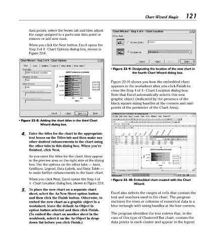
• Figure 22-9: Designating the location of the new chart in
the fourth Chart Wizard dialog box.

Figure 22-10 shows you how the embedded chart
appears in the worksheet after you click Finish to
close the Step 4 of 4 - Chart Location dialog box.
Note that Excel automatically selects this new
graphic object (indicated by the presence of the
black square sizing handles at the corners and mid-
points of the perimeter of the Chart Area).

• Figure 22-8: Adding the chart titles in the third Chart
Wizard dialog box.

4. Enter the titles for the chart in the appropriate
text boxes on the Titles tab and then make any
other desired enhancements to the chart using
the other tabs in this dialog box. When you’re
finished, click Next.
As you enter the titles for the chart, they appear
in the preview area on the right side of the dialog
box. Use the options on the other tabs — Axes,
Gridlines, Legend, Data Labels, and Data Table —
to make further enhancements to the basic chart.
When you click Next, Excel opens the Step 4 of • Figure 22-10: Embedded chart created with the Chart
4 - Chart Location dialog box, shown in Figure 22-9. Wizard.
5. To place the new chart on a separate chart
sheet, select the As New Sheet option button Excel also selects the ranges of cells that contain the
and then click the Finish button. Otherwise, to text and numbers used in the chart. The program
embed the new chart as a graphic object in a encloses the rows or columns of numerical data in a
worksheet, leave the default As Object In blue rectangle with sizing handles at the four corners.
option button selected and then click Finish.
(To embed the chart on another sheet in the The program identifies the text entries that, in the
workbook, select it on the As Object In drop- case of this type of Clustered Bar chart, contain the
down list before you click Finish.) data points in each cluster and appear in the legend