Page 26 - Finite Element Modeling and Simulations with ANSYS Workbench

Introduction 11

 100 − 100
k 3 =  −  (N/mm )
 100 100 

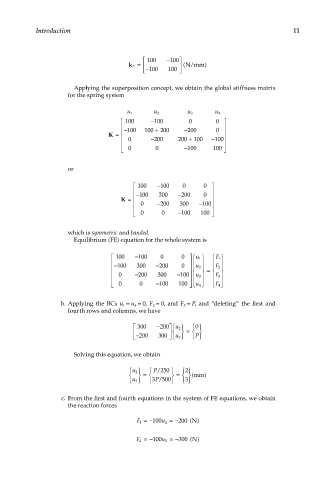
Applying the superposition concept, we obtain the global stiffness matrix
for the spring system

u 1 u 2 u 3 u 4
 100 − 100 0 0 
 − 100 100 + 200 − 200 0 
K =  
 0 − 200 200 + 100 − 100
 − 
  0 0 100 1000  

or

 100 −100 0 0 
 −100 300 −200 0 
K =  
 0 −200 300 −100 
 
  0 0 −100 100  

which is symmetric and banded.
Equilibrium (FE) equation for the whole system is

 100 − 100 0 0  u   F 1 

1
 − −    
F 2

 100 300 200 0   u u 2  =  

 0 − 200 300 − 100 u 3   

F 3
 −     

  0 0 100 100  u 4   F 4 
b. Applying the BCs u 1 = u 4 = 0, F 2 = 0, and F 3 = P, and “deleting” the first and
fourth rows and columns, we have
 300 − 200u 2   0
 −    =  
P
 200 300  u 3     
Solving this equation, we obtain
 u 2   /  2
P 250 
  =   =   (mm)
P 500 
3 
 u 3    3 /   
c. From the first and fourth equations in the system of FE equations, we obtain
the reaction forces
N
F 1 =− 100 u 2 =− 200 ()

N
F 4 =− 100 u 3 =− 300 ()