Page 23 - Finite Element Modeling and Simulations with ANSYS Workbench

8 Finite Element Modeling and Simulation with ANSYS Workbench

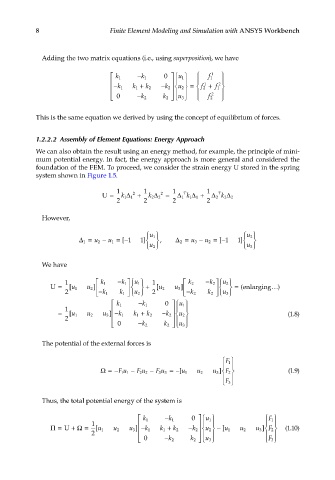
Adding the two matrix equations (i.e., using superposition), we have

 k 1 − k 1 0  u 1   f 1 1 
 − k 1 + −     f 2 + 2 
1

 k 1 k 2 k 2  u 2 =  f 1 
1



 0 − k 2  u 3   2 f 2 
 k 2  
This is the same equation we derived by using the concept of equilibrium of forces.
1.2.2.2 Assembly of Element Equations: Energy Approach
We can also obtain the result using an energy method, for example, the principle of mini-
mum potential energy. In fact, the energy approach is more general and considered the
foundation of the FEM. To proceed, we consider the strain energy U stored in the spring
system shown in Figure 1.5.

1 1 1 1
T
U = 1 k ∆ 1 2 + 2 k ∆ 2 2 = ∆ 1 k ∆ 1 + ∆ 2 k ∆ 2
T
1
2
2 2 2 2
However,
u 1 u 2 
∆ 1 = u 2 − u 1 =−[ 1 1  ]  , ∆ 2 = u 3 − u 2 =−[ 1 1  ] 
 u 2   u 3 

We have

1 k

1  k 1 −  1 u  1  k 2 − 2 k u 2 
U = [u 1 u 2 ]     + [u 2 u 3 ]     = (enlarging …)
u
2  − 1 k 1 k  2 u  2  − 2 k 2 k  3 
 k 1 −k 1 0  1 u 
1   
= [ u 1 u 2 u 3 ] −k 1 k 1 + k 2 −k 2  2 u  (1.8)
2     
 0 −k 2 2 2 k   3 u 
The potential of the external forces is

 
F 1
[
Ω= −Fu − Fu − Fu = − u 1 u 2 u 3 ]   (1.9)
 
F 2
22
11
33
 
F 3
 
Thus, the total potential energy of the system is
 k 1 − 1 k 0  1 u   
F 1
1     
Π = U + Ω = [u 1 2 u u 3 ] − 1 k 1 k + k 2 − 2 k  2 u  − [u 1 u 2 u 3 ] F 2 (1.10)
 
2      



F 3
 0 − 2 k 2 k  u 3   