Page 99 - Finite Element Modeling and Simulations with ANSYS Workbench

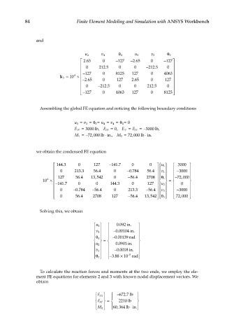
84 Finite Element Modeling and Simulation with ANSYS Workbench

and

4 θ 2 θ
u 4 v 4 u 2 v 2
 265 0 − 127 − . 0 − 127
265
.
 
 0 212 5 . 0 0 − 212 5 . 0 
 − 127 0 8 8125 127 0 4063
4
k 3 = 10 ×  
.
265
 − . 0 127 265 0 127 
 0 − 212 5 . 0 0 212 5 . 0 
 
  − 127 0 4063 127 0 8 8125  
Assembling the global FE equation and noticing the following boundary conditions
u 3 = v 3 = θ= u 4 = v 4 = θ= 0
4
3
F X1 = 3000 lb, F X2 = 0, F Y1 = F Y2 = − 3000 lb,
⋅
M 1 =− 72,,000 lb in. , M 2 = 72 ,000 lbin .
⋅

we obtain the condensed FE equation

 144 3 . 0 127 − 141 7 . 0 0 u 1   3000 
    
0 784
 0 213 3 . 564 . 0 − . 56 4 .  1 v   −3000 
 127 56 4 . 13 542 0 − 5664 . 2708  θ   −72 000 

,
,

1 


4
10 ×      =  
 − 141 7 . 0 0 144 3 . 0 127   2 u   0  
 0 − 0 784 − 56 4 . 0 213 3 . − 564 .   2 v   −3000 
.
     
 
,
2 
  0 564 . 2708 1227 − 56 4 . 13 542 θ    72 000,  
Solving this, we obtain
.
 u 1   0 092 in. 
   
0 00104 in.
 v 1   − . 
 1 θ     − 00 . 00139 rad  

  =  
.
 u 2   0 0901in.  
 v 2   − 0 0018 in. 
.
   − 5 
.
  2 θ     − 388 × 10 rad  
To calculate the reaction forces and moments at the two ends, we employ the ele-
ment FE equations for elements 2 and 3 with known nodal displacement vectors. We
obtain
 F X3   − 672 7 . lb 
   
 F Y3  =  2210 lb 
   60 364 lb in . 
⋅
,
 M 3   