Page 95 - Finite Element Modeling and Simulations with ANSYS Workbench

80 Finite Element Modeling and Simulation with ANSYS Workbench

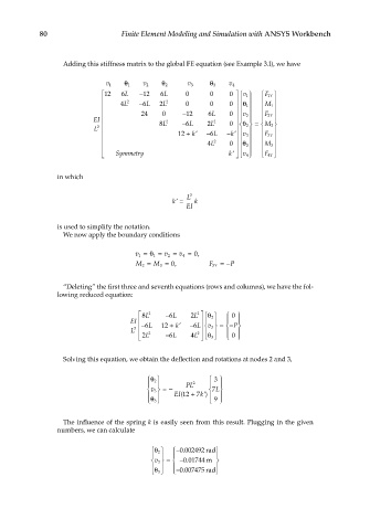
Adding this stiffness matrix to the global FE equation (see Example 3.1), we have

1 θ 2 θ 3 θ
v 1 v 2 v 3 v 4

 12 6 L − 12 6 L 0 0 0  v   1 F Y 
1
 2 − 2    
 4 L 6 L 2 L 0 0 0  1 θ   M 1 
 24 0 − 12 6 L 0  v   2 F Y 

2
EI  8 L 2 − 6 L 2 L 2 0  θ 2 =   M 2 


L 3   −    2   
2
 12 + k’ 6L −k’ v 3   3 F Y 


 4L 2 0  θ    M 3 
3
 Symmetry k’    
  4 v   4 F Y 
in which
L 3
k’ = k
EI
is used to simplify the notation.
We now apply the boundary conditions
v 1 =θ = v 2 = v 4 = 0,
1
M 2 = M 3 = 0, F Y3 =− P

“Deleting” the first three and seventh equations (rows and columns), we have the fol-
lowing reduced equation:


2
 8 L 2 − 6 L 2 L  θ   0 
EI  − 12 + −  2   
 P

L 3   6 L − k’ 6 L  v 3  =−  

2  
 
2
 2 L 6 L 4 L   3 θ   0 
Solving this equation, we obtain the deflection and rotations at nodes 2 and 3,
θ   3 
 2
  PL 2  
 3 v  =−  7L 
  EI( 12 + 7k’)  9 
 θ 3   
The influence of the spring k is easily seen from this result. Plugging in the given
numbers, we can calculate

θ   −0 002492. rad 
 2
   
 3 v  =  −0 01744. m 
   −0 007475. rad 
 θ 3    