Page 93 - Finite Element Modeling and Simulations with ANSYS Workbench

78 Finite Element Modeling and Simulation with ANSYS Workbench

Solution
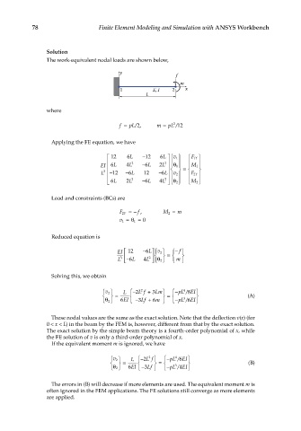
The work-equivalent nodal loads are shown below,
y f

m
1 E, I 2 x
L

where

f = pL/, m = pL /12
2
2

Applying the FE equation, we have

 12 6 L − 12 6 L   F Y 
v 1
1

EI 6 L 4 L 2 − 6 L 2 L 2     
θ 


 1
 M 1
  = 
L  − 12 − 6 L 12 − 6 L v 2  F Y  
3
 
2
 2 − L  θ  
2 


 M 2
2
  6 L 2 L 6 L 4    
Load and constraints (BCs) are
F Y2 =− , M 2 = m
f
v 1 =θ = 0
1
Reduced equation is
EI  12 − 6 L   − f 
v 2
L 3   − 6 L 4 L 2    =   m   
2 θ 
 

Solving this, we obtain
2
4
 v 2  L   − 2 Lf + 3 Lm    − pL 8 / EI 
  = 6  − Lf +  =  − 3  (A)
I
2 θ 

  EI  3 6 m     pL 6 / EI  
These nodal values are the same as the exact solution. Note that the deflection v(x) (for
0 < x < L) in the beam by the FEM is, however, different from that by the exact solution.
The exact solution by the simple beam theory is a fourth-order polynomial of x, while
the FE solution of v is only a third-order polynomial of x.
If the equivalent moment m is ignored, we have
 v 2  L   − 2 Lf     − pL 6 / EI  
4
2
  = 6  −  =  − 3   (B)
2 θ 
/

  EI  3 Lf     pL 4 EI  
The errors in (B) will decrease if more elements are used. The equivalent moment m is
often ignored in the FEM applications. The FE solutions still converge as more elements
are applied.