Page 89 - Finite Element Modeling and Simulations with ANSYS Workbench

74 Finite Element Modeling and Simulation with ANSYS Workbench

We conclude that the stiffness matrix for the simple beam element is

L
T
k = ∫ B EI dx (3.10)
B
0
Applying the result in Equation 3.10 and carrying out the integration, we arrive at the
same stiffness matrix as given in Equation 3.5.

3.4.3 Treatment of Distributed Loads
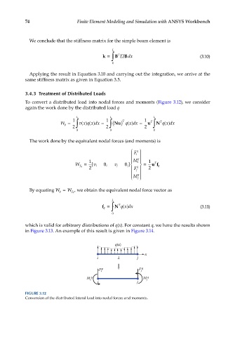
To convert a distributed load into nodal forces and moments (Figure 3.12), we consider
again the work done by the distributed load q

L L L
1 1 T 1
W q = ∫ vxqxdx = ∫ (Nu ) q xdx = u T ∫ N T q xdx
()
()
()
()
2 2 2
0 0 0
The work done by the equivalent nodal forces (and moments) is
 F 
q
i
 
q
1  M  1
i
= [ i θ  = uf
T
W f q v i v j j θ  ] q q
2  F j  2
 M q
 j 
By equating W q = W f q , we obtain the equivalent nodal force vector as
L
f q = ∫ N qx dx (3.11)
T
()
0
which is valid for arbitrary distributions of q(x). For constant q, we have the results shown
in Figure 3.13. An example of this result is given in Figure 3.14.

q(x)
x
i L j

F i q F j q

M i q M j q
i j

FIGURE 3.12
Conversion of the distributed lateral load into nodal forces and moments.