Page 86 - Finite Element Modeling and Simulations with ANSYS Workbench

Beams and Frames 71

y
v , F i v , F j
i
j
i j
E,I x
, M i , M j
i
j
L
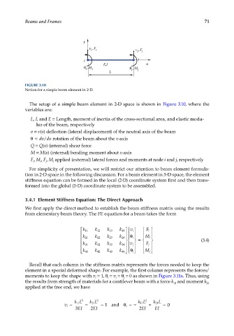
FIGURE 3.10
Notion for a simple beam element in 2-D.

The setup of a simple beam element in 2-D space is shown in Figure 3.10, where the
variables are:
L, I, and E = Length, moment of inertia of the cross-sectional area, and elastic modu-
lus of the beam, respectively
v = v(x) deflection (lateral displacement) of the neutral axis of the beam
θ= dv dx rotation of the beam about the z-axis
/
Q = Q(x) (internal) shear force
M = M(x) (internal) bending moment about z-axis
F, M , F, M applied (external) lateral forces and moments at node i and j, respectively
j
j
i
i
For simplicity of presentation, we will restrict our attention to beam element formula-
tion in 2-D space in the following discussion. For a beam element in 3-D space, the element
stiffness equation can be formed in the local (2-D) coordinate system first and then trans-
formed into the global (3-D) coordinate system to be assembled.

3.4.1 Element Stiffness Equation: The Direct Approach
We first apply the direct method to establish the beam stiffness matrix using the results
from elementary beam theory. The FE equation for a beam takes the form

 k 11 k 12 k 13 k 14    F i 
v i
    
 k 21 k 22 k 23 k 24    M i  (3.4)

θ i

  = 
 k 31 k 32 k 33 k 34   v j F j
     
θ 


M j
j
 k 41 k 42 k 43 k 44    
Recall that each column in the stiffness matrix represents the forces needed to keep the
element in a special deformed shape. For example, the first column represents the forces/
moments to keep the shape with v = 1, θ = v = θ = 0 as shown in Figure 3.11a. Thus, using
i
i
j
j
the results from strength of materials for a cantilever beam with a force k and moment k
21
11
applied at the free end, we have
kL 3 kL 2 kL 2 kL
v i = 11 − 21 = 1 and i θ =− 11 + 21 = 0
3 EI 2 EI 2 EI EI