Page 383 - Fluid-Structure Interactions Slender Structure and Axial Flow (Volume 1)

PIPES CONVEYING FLUID: NONLINEAR AND CHAOTIC DYNAMICS 359

20. . 1 . . ? ' . . ,...-.-..- 20 .... I . - -
15 u = 8.025
- 10 -
c- 10
h
v
'F 5
d
.- 0-
x
- o
s -5 -10 -
-10
-15 . .' .. ' .'.'..-. -20 . ' . . '. . . .
-1.0 -0.5 0.0 0.5 1.0 1.5 -1.5 -1.0 4.5 0.0 0.5 1.0 1.5
(C) (d)
Displacement, q(1,~)

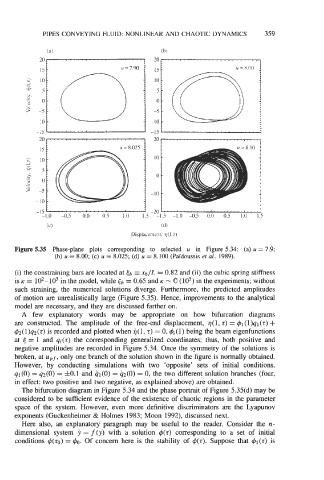
Figure 5.35 Phase-plane plots corresponding to selected u in Figure 5.34: (a) u = 7.9;
(b) u = 8.00; (c) u = 8.025; (d) u = 8.100 (PaYdoussis et al. 1989).

(i) the constraining bars are located at <b xb/L = 0.82 and (ii) the cubic spring stiffness
is K = 102-103 in the model, while <b = 0.65 and K - 6 (lo5) in the experiments; without
such straining, the numerical solutions diverge. Furthermore, the predicted amplitudes
of motion are unrealistically large (Figure 5.35). Hence, improvements to the analytical
model are necessary, and they are discussed farther on.
A few explanatory words may be appropriate on how bifurcation diagrams
are constructed. The amplitude of the free-end displacement, ~(1, = $l(l)ql(t) +
t)
&(l)q2(t) is recorded and plotted when rj(1, t) = 0, &(l) being the beam eigenfunctions
at 6 = 1 and qi(t) the corresponding generalized coordinates; thus, both positive and
negative amplitudes are recorded in Figure 5.34. Once the symmetry of the solutions is
broken, at upf, only one branch of the solution shown in the figure is normally obtained.
However, by conducting simulations with two 'opposite' sets of initial conditions,
41 (0) = q2(0) = fO. 1 and ql(0) = &(O) = 0, the two different solution branches (four,
in effect: two positive and two negative, as explained above) are obtained.
The bifurcation diagram in Figure 5.34 and the phase portrait of Figure 5.35(d) may be
considered to be sufficient evidence of the existence of chaotic regions in the parameter
space of the system. However, even more definitive discriminators are the Lyapunov
exponents (Guckenheimer & Holmes 1983; Moon 1992), discussed next.
Here also, an explanatory paragraph may be useful to the reader. Consider the n-
dimensional system y = f(y) with a solution $(t) corresponding to a set of initial
conditions 4(t0) = $0. Of concern here is the stability of $(t). Suppose that $l(t) is