Page 385 - Fluid-Structure Interactions Slender Structure and Axial Flow (Volume 1)

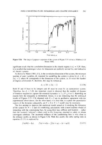
PIPES CONVEYING FLUID: NONLINEAR AND CHAOTIC DYNAMICS 361

2.0

1 .5

I .0

0.5

0.0
8.027
-0.5 . . * * f . . . . I . * .f'*.'"""".
7.90 7.95 8.00 8.05 8.10 8.15 8.20
Fluid velocity, u

Figure 5.36 The largest Lyapunov exponent of the system of Figure 5.34 versus u (Paidoussis &
Moon 1988).

significant result: that the correlation dimension in the chaotic regime is d, = 3.20. Here,
it is recalled that noninteger values for dimension are perfectly normal for, and indicative
of, chaotic systems.
As shown by MaiiC (198 l), if d, is the correlation dimension of the system, the minimum
number of state variables, M, required for modelling the system is given by d, 5 M I
2d, + 2, where M corresponds to the dimension of the system, i.e. to twice the number
of degrees of freedom N; therefore, this may be written as
d, 5 2N 5 2d, + 2. (5.136)

Both M and N have to be integers and M must be even for an autonomous system.
Therefore, for d, = 3.20, the important result is obtained that the number of degrees
of freedom required to capture the essential dynamics is 2 5 N 5 4 or 5, depending on
exactly how the inequality is interpreted. Hence, it is not surprising that the analytical
results of Figures 5.33-5.36 obtained with N = 2 are in qualitative agreement with the
experimental observations. On the other hand, it is clear that, to capture the quantitative
aspects of the dynamics adequately, an N = 4 or N = 5 model may be necessary.
The first attempt to improve the analytical model aimed at (i) studying the dynamics
of the system for N > 2 and (ii) conducting calculations with a more realistic model of
impacting with the constraining bars, by using their true stiffness and location - rather
than the strained ('relaxed') values used in the foregoing, resorted to solely to obtain
convergent solutions. The measured stiffness of the constraining bars is very close to
the trilinear model, as shown in Figure 5.38. With this model, the cubic spring term in
equation (5.131) is replaced by

f(q>s($ - (b), f(q) = K{q - $(lq + qbl - Ir - qbl)}. (5.137)