Page 406 - Fluid-Structure Interactions Slender Structure and Axial Flow (Volume 1)

382 SLENDER STRUCTURES AND AXIAL FLOW

For ug = 3.164 (Copeland & Moon 1992; Figure 9), the phase-plane plot becomes
completely irregular, the Poincark section shows an unstructured cloud of points, while
in the power spectrum the low-frequency background level has risen to almost drown the
subharmonic combination peaks, all indicating that the motion is chaotic.
In the analysis (Copeland 1992), motions in both the (x, y) and (x, z) planes are
considered - cf. Figure 5.2(b). To simplify things, because the pipes used in the exper-
iments are so slender and flexible, the flexural restoring forces are much smaller than
the gravity-induced tensile forces and they are neglected. Thus, the equation of motion
is reduced to that of a pipe-string with an end-mass. This is the reason for defining
ug = U/(gL)'/* such that it does not involve EZ. Furthermore, the effect of the end-mass
is not incorporated in the equation of motion but is left in the boundary conditions. Thus,
the system is discretized using specially determined comparison functions for a heavy
string with an end-mass, involving Bessel functions, to proceed with the analysis.
The linearized system is found to lose stability in its third and fourth modes succes-
sively by Hopf bifurcations - of multiplicity two, for each of the two lateral directions.
Two reduced forms of the discretized nonlinear system are then analysed: (i) an eight-
dimensional invariant manifold, consisting of four centre eigendirections (associated with
the two symmetric modes, the third and fourth, first undergoing a Hopf bifurcation) and
four stable eigendirections, is obtained and solved numerically; (ii) the further reduced,
four-dimensional centre manifold involving but the centre space of the eight-dimensional
one, which is analysed further. Then, proceeding essentially as in Appendices F and H via
the method of averaging, and assessing stability in the same manner as in Section 5.7.2,
the nature of the Hopf bifurcation may be determined (whether sub- or supercritical)
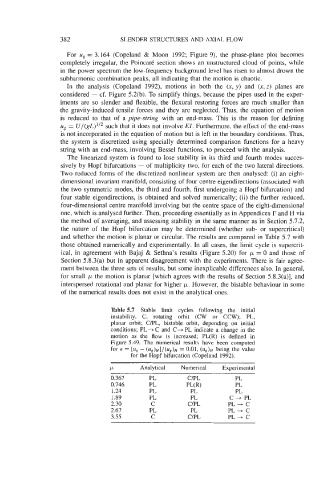
and whether the motion is planar or circular. The results are compared in Table 5.7 with
those obtained numerically and experimentally. In all cases, the limit cycle is supercrit-
ical, in agreement with Bajaj & Sethna's results (Figure 5.20) for p = 0 and those of
Section 5.8.3(a) but in apparent disagreement with the experiments. There is fair agree-
ment between the three sets of results, but some inexplicable differences also. In general,
for small p the motion is planar [which agrees with the results of Section 5.8.3(a)], and
interspersed rotational and planar for higher p. However, the bistable behaviour in some
of the numerical results does not exist in the analytical ones.

Table 5.7 Stable limit cycles following the initial
instability. C, rotating orbit (CW or CCW); PL,
planar orbit; CPL, bistable orbit, depending on initial
conditions; PL-2 C and C+ PL indicate a change in the
motion as the flow is increased; PL(R) is defined in
Figure 5.49. The numerical results have been computed
for E = [ue - (U~)~]/(U~)~ 0.01, (uR)~ being the value
=
for the Hopf bifurcation (Copeland 1992).
P Analytical Numerical Experimental
0.367 PL CIPL PL
0.746 PL PL(R) PL
1.24 PL PL PL
1.89 PL PL c + PL
2.30 C CPL PL -2 c
2.67 PL PL PL + c
3.55 C CPL PL + c