
Page 401 - Fluid-Structure Interactions Slender Structure and Axial Flow (Volume 1)
P. 401
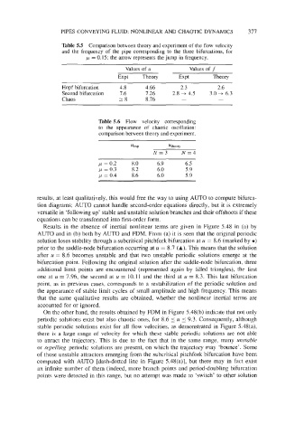
PIPES CONVEYING FLUID: NONLINEAR AND CHAOTIC DYNAMICS          377

                      Table 5.5  Comparison between theory and experiment of  the flow velocity
                      and  the  frequency of  the  pipe  corresponding  to  the  three  bifurcations,  for
                              p = 0.15; the arrow represents the jump in frequency.

                                           Values of  u         Values of  f
                                         Expt    Theory      Expt       Theory

                      Hopf bifurcation   4.8      4.66        2.3         2.6
                      Second bifurcation   7.6    7.26     2.8 + 4.5   3.0 + 6.3
                      Chaos              -8       8.76        -           -


                                  Table 5.6  Flow  velocity  corresponding
                                  to  the  appearance  of  chaotic  oscillation:
                                  comparison between theory and experiment.

                                             Uexp        Utheory
                                                    N=3       N=4
                                  p = 0.2    8.0      6.9      6.5
                                  p = 0.3    8.2      6.0      5.9
                                  p = 0.4    8.6      6.0      5.9


              results, at least qualitatively, this would free the way to using AUTO to compute bifurca-
              tion diagrams;  AUTO cannot handle second-order equations directly, but it is extremely
              versatile in ‘following up’ stable and unstable solution branches and their offshoots if these
              equations can be transformed into first-order form.
                Results  in  the  absence of  inertial  nonlinear  terms  are given  in  Figure 5.48 in  (a) by
              AUTO and in (b) both by AUTO and FDM. From (a) it is seen that the original periodic
              solution loses stability through a subcritical pitchfork bifurcation at u = 8.6 (marked by  0)
              prior to the saddle-node bifurcation occurring at u = 8.7 (A). This means that the solution
              after  u = 8.6 becomes  unstable  and  that  two  unstable  periodic  solutions emerge  at  the
             bifurcation point. Following the original solution after the saddle-node bifurcation, three
              additional  limit  points  are  encountered  (represented  again  by  filled triangles),  the  first
              one at  u = 7.96, the  second at  u = 10.11 and the third at u = 8.3. This last bifurcation
              point,  as in previous cases, corresponds  to  a restabilization  of  the periodic  solution and
              the appearance of  stable limit cycles of  small amplitude and high frequency. This means
              that  the  same  qualitative  results  are  obtained,  whether  the  nonlinear  inertial  terms  are
              accounted for or ignored.
                On the other hand, the results obtained by FDM in Figure 5.48(b) indicate that not only
              periodic  solutions exist but also chaotic ones, for 8.6 5 u 5 9.3. Consequently, although
              stable periodic  solutions exist for all flow  velocities, as demonstrated  in  Figure 5.48(a),
              there  is a large range  of  velocity for which  these  stable periodic  solutions are not  able
              to  attract  the  trajectory.  This  is  due to  the  fact that  in  the  same range,  many  unstable
             or repelling  periodic solutions are present, on which the trajectory may  ‘bounce’. Some
             of  those unstable attractors emerging from the subcritical pitchfork bifurcation have been
             computed  with  AUTO  [dash-dotted line in  Figure 5.48(a)], but  there  may  in  fact  exist
              an infinite number of them (indeed, more branch points and period-doubling bifurcation
              points were detected in this range, but no attempt was made to  ‘switch’ to other solution