Page 399 - Fluid-Structure Interactions Slender Structure and Axial Flow (Volume 1)

PIPES CONVEYING FLUID: NONLINEAR AND CHAOTIC DYNAMICS 375

again. Furthermore, there is a frequency jump in the periodic oscillations in the theoret-
ical results before and after the quasiperiodic band: f = w/2n = 3.1 for u = 8.0 versus
f = 6.5 for u = 8.8. This corresponds to the jump observed across the second bifurcation
in the experiments, Figure 5.45(b), but only at higher values of p.
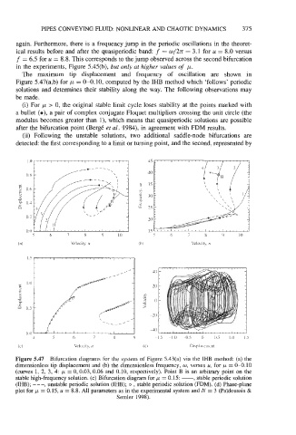
The maximum tip displacement and frequency of oscillation are shown in
Figure 5.47(a,b) for p = 0-0.10, computed by the IHB method which ‘follows’ periodic
solutions and determines their stability along the way. The following observations may
be made.
(i) For p > 0, the original stable limit cycle loses stability at the points marked with
a bullet (o), a pair of complex conjugate Floquet multipliers crossing the unit circle (the
modulus becomes greater than l), which means that quasiperiodic solutions are possible
after the bifurcation point (Berg6 et al. -1984), in agreement with FDM results.
(ii) Following the unstable solutions, two additional saddle-node bifurcations are
detected: the first corresponding to a limit or turning point, and the second, represented by

5 6 I 8 9 10
(a) Velocity, u Velocity, u

1.5

* 1.0
D
-
n
B
.-
0 0.5

0.0
4 5 6 I 8 9 -1.5 -1.0 -0.5 0 0.5 1.0 1.5
(C) Velocity, u ld) Displacement
Figure 5.47 Bifurcation diagrams for the system of Figure 5.43(a) via the IHB method: (a) the
dimensionless tip displacement and (b) the dimensionless frequency, w, versus u, for p = 0-0.10
(curves 1, 2, 3, 4: p = 0,0.03,0.06 and 0.10, respectively). Point B is an arbitrary point on the
stable high-frequency solution. (c) Bifurcation diagram for p = 0.15: -, stable periodic solution
(IHB); - - -, unstable periodic solution (IHB); o , stable periodic solution (FDM). (d) Phase-plane
plot for p = 0.15, u = 8.8. All parameters as in the experimental system and N = 3 (Pdidoussis &
Semler 1998).