Page 167 - T. Anderson-Fracture Mechanics - Fundamentals and Applns.-CRC (2005)

1656_C003.fm Page 147 Monday, May 23, 2005 5:42 PM

Elastic-Plastic Fracture Mechanics 147

where J is the effective small-scale yielding J, i.e., the value of J that would result in the area
o
A(s /s ) if the structure were large relative to the plastic zone, and T = Q = 0. Therefore, the ratio
o
1
of the applied J to the effective J is given by
J = 1 (3.83)
J o φ

The small-scale yielding J value (J ) can be viewed as the effective driving force for cleavage,
o
while J is the apparent driving force.
The J/J ratio quantifies the size dependence of cleavage fracture toughness. Consider, for
o
example, a finite size test specimen that fails at J = 200 kPa m. If the J/J ratio were 2.0 in this
o
c
case, a very large specimen made from the same material would fail at J = 100 kPa m. An equivalent
c
toughness ratio in terms of the crack-tip-opening displacement (CTOD) can also be defined.

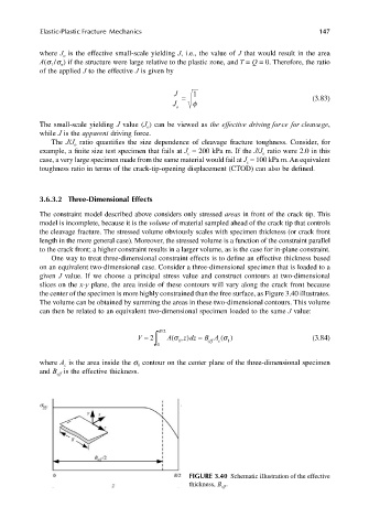
3.6.3.2 Three-Dimensional Effects
The constraint model described above considers only stressed areas in front of the crack tip. This
model is incomplete, because it is the volume of material sampled ahead of the crack tip that controls
the cleavage fracture. The stressed volume obviously scales with specimen thickness (or crack front
length in the more general case). Moreover, the stressed volume is a function of the constraint parallel
to the crack front; a higher constraint results in a larger volume, as is the case for in-plane constraint.
One way to treat three-dimensional constraint effects is to define an effective thickness based
on an equivalent two-dimensional case. Consider a three-dimensional specimen that is loaded to a
given J value. If we choose a principal stress value and construct contours at two-dimensional
slices on the x-y plane, the area inside of these contours will vary along the crack front because
the center of the specimen is more highly constrained than the free surface, as Figure 3.40 illustrates.
The volume can be obtained by summing the areas in these two-dimensional contours. This volume
can then be related to an equivalent two-dimensional specimen loaded to the same J value:

σ
V ∫ B 2 / A = z d (, ) z σ = 2 B eff A c ( ) (3.84)
0 1 1

where A is the area inside the s contour on the center plane of the three-dimensional specimen
c
1
and B is the effective thickness.
eff

FIGURE 3.40 Schematic illustration of the effective
thickness, B eff .