Page 168 - T. Anderson-Fracture Mechanics - Fundamentals and Applns.-CRC (2005)

1656_C003.fm Page 148 Monday, May 23, 2005 5:42 PM

148 Fracture Mechanics: Fundamentals and Applications

The effective thickness influences the cleavage driving force through a sample volume effect: longer
crack fronts have a higher probability of cleavage fracture because more volume is sampled along the
crack front. This effect can be characterized by a three-parameter Weibull distribution (See Chapter 5):

 B K  K −  4 
1

F =− exp −  B  Θ JC − K min   (3.85)
 o  K min   
where
B = thickness (or crack front length)
B = reference thickness
o
K = threshold toughness
min
Θ = 63rd percentile toughness when B = B o
K
Consider two samples with effective crack front lengths B and B . If a value of K is measured
1 2 JC(1)
for Specimen 1, the expected toughness for Specimen 2 can be inferred from Equation (3.85) by
equating failure probabilities:

 B  / 14
K = 1 K − K ( min) + K (3.86)
2
JC()   B   JC() 1 min
2
Equation (3.86) is a statistical thickness adjustment that can be used to relate two sets of data with
different thicknesses.

3.6.3.3 Application of the Model
As with the J-Q approach, the implementation of the scaling model requires detailed elastic-plastic
finite element analysis of the configuration of interest. The principal stress contours must be con-
structed and the areas compared with the T = 0 reference solution obtained from a modified boundary
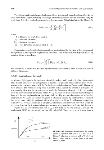
layer analysis. The effective driving force J is then plotted against the applied J, as Figure 3.41
o
schematically illustrates. At low deformation levels, the J -J curves follow the 1:1 line, but deviate
o
from the line with further deformation. When ≈ J o , the crack-tip stress fields are close to the Q = 0
J
limit, and fracture toughness is not significantly influenced by specimen boundaries. At high defor-
mation levels J > J and the fracture toughness is artificially elevated by constraint loss. Constraint
o
loss occurs more rapidly in specimens with shallow cracks, as Figure 3.28 illustrates. A specimen
with a/W = 0.15 would tend to fail at a higher J value than a specimen with a/W = 0.5. Given the
c
J -J curve, however, the J values for both specimens can be corrected to J , as Figure 3.41 illustrates.
o
o
c
Figure 3.42 is a nondimensional plot of J at the midplane vs. the average J through the
o
thickness of SENB specimens with various W/B ratios [36]. These curves were inferred from a

FIGURE 3.41 Schematic illustration of the scaling
model. A specimen with a/W = 0.15 will fail at a
higher J c value than a specimen with a/W = 0.5, but
both J c values can be corrected down to the same
critical J o value.