Page 172 - T. Anderson-Fracture Mechanics - Fundamentals and Applns.-CRC (2005)

1656_C003.fm Page 152 Monday, May 23, 2005 5:42 PM

152 Fracture Mechanics: Fundamentals and Applications

The exponents s and the angular functions for each term in the series can be determined from the
k
asymptotic analysis. The amplitudes for the first five terms are as follows:

 − 1 + 
 A   I () n 1 
n
1
 A    (unspecified )  
 2  A 2
 A  =   2  
 3  A 1
 A 4    (unspecified )  
  A   A 2 3 
5
  A 1 2  

The two unspecified coefficients A and A are governed by the far-field boundary conditions. The
4
2
first five terms of the series have three degrees of freedom, where J, A , and A are independent
2
4
parameters. For low and moderate strain hardening materials, Crane [43] showed that a fourth
independent parameter does not appear in the series for many terms. For example, when n = 10,
the fourth independent coefficient appears in approximately the 100th term. Thus for all practical
purposes, the crack-tip stress field inside the plastic zone has three degrees of freedom.
Since two-parameter theories assume two degrees of freedom, they cannot be rigorously correct
in general. There are, however, situations where two-parameter approaches provide a good engineering
approximation.
Consider the modified boundary layer model in Figure 3.32. Since the boundary conditions
have only two degrees of freedom (K and T), the resulting stresses and strains inside the plastic
zone must be two-parameter fields. Thus there must be a unique relationship between A and A in
4
2
this case. That is
A A = A ( ) (3.88)
4 4 2
The two-parameter theory is approximately valid for other geometries to the extent that the
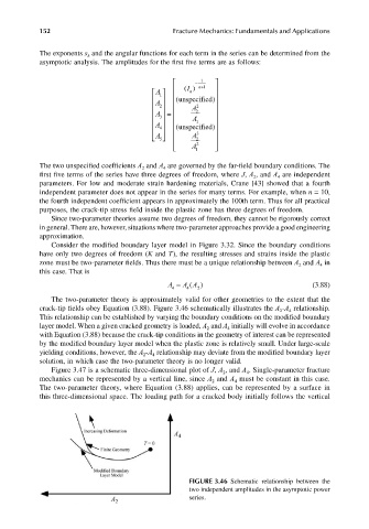
crack-tip fields obey Equation (3.88). Figure 3.46 schematically illustrates the A -A relationship.
4
2
This relationship can be established by varying the boundary conditions on the modified boundary
layer model. When a given cracked geometry is loaded, A and A initially will evolve in accordance
2
4
with Equation (3.88) because the crack-tip conditions in the geometry of interest can be represented
by the modified boundary layer model when the plastic zone is relatively small. Under large-scale
yielding conditions, however, the A -A relationship may deviate from the modified boundary layer
2
4
solution, in which case the two-parameter theory is no longer valid.
Figure 3.47 is a schematic three-dimensional plot of J, A , and A . Single-parameter fracture
4
2
mechanics can be represented by a vertical line, since A and A must be constant in this case.
2
4
The two-parameter theory, where Equation (3.88) applies, can be represented by a surface in
this three-dimensional space. The loading path for a cracked body initially follows the vertical

FIGURE 3.46 Schematic relationship between the
two independent amplitudes in the asymptotic power
series.