Page 237 - Fundamentals of Gas Shale Reservoirs

MICROSEISMIC DOWNHOLE MONITORING 217

1.653.600 1.654.600 1.655.600
289.000
288.500
288.000

287.500

287.000
Monitoring 286.500
well
1.500
286.000
Treatment
well 2.000
285.500
Treatment
well 2.500
285.000
Monitoring 3.000
284.500 well
3.500
284.000
4.000
N 283.500 N E 4.500
–500
E Z
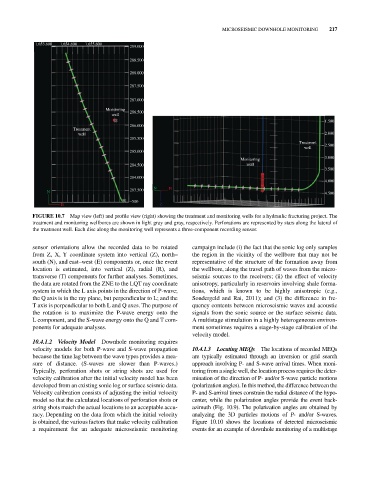
FIGURE 10.7 Map view (left) and profile view (right) showing the treatment and monitoring wells for a hydraulic fracturing project. The
treatment and monitoring wellbores are shown in light gray and gray, respectively. Perforations are represented by stars along the lateral of
the treatment well. Each disc along the monitoring well represents a three‐component recording sensor.

sensor orientations allow the recorded data to be rotated campaign include (i) the fact that the sonic log only samples
from Z, X, Y coordinate system into vertical (Z), north– the region in the vicinity of the wellbore that may not be
south (N), and east–west (E) components or, once the event representative of the structure of the formation away from
location is estimated, into vertical (Z), radial (R), and the wellbore, along the travel path of waves from the micro­
transverse (T) components for further analyses. Sometimes, seismic sources to the receivers; (ii) the effect of velocity
the data are rotated from the ZNE to the LQT ray coordinate anisotropy, particularly in reservoirs involving shale forma­
system in which the L axis points in the direction of P‐wave; tions, which is known to be highly anisotropic (e.g.,
the Q axis is in the ray plane, but perpendicular to L; and the Sondergeld and Rai, 2011); and (3) the difference in fre­
T axis is perpendicular to both L and Q axes. The purpose of quency contents between microseismic waves and acoustic
the rotation is to maximize the P‐wave energy onto the signals from the sonic source or the surface seismic data.
L component, and the S­wave energy onto the Q and T com­ A multistage stimulation in a highly heterogeneous environ­
ponents for adequate analyses. ment sometimes requires a stage‐by‐stage calibration of the
velocity model.
10.4.1.2 Velocity Model Downhole monitoring requires
velocity models for both P‐wave and S‐wave propagation 10.4.1.3 Locating MEQs The locations of recorded MEQs
because the time lag between the wave types provides a mea­ are typically estimated through an inversion or grid search
sure of distance. (S‐waves are slower than P‐waves.) approach involving P‐ and S‐wave arrival times. When moni­
Typically, perforation shots or string shots are used for toring from a single well, the location process requires the deter­
velocity calibration after the initial velocity model has been mination of the direction of P‐ and/or S‐wave particle motions
developed from an existing sonic log or surface seismic data. (polarization angles). In this method, the difference between the
Velocity calibration consists of adjusting the initial velocity P‐ and S‐arrival times constrain the radial distance of the hypo­
model so that the calculated locations of perforation shots or center, while the polarization angles provide the event back‐
string shots match the actual locations to an acceptable accu­ azimuth (Fig. 10.9). The polarization angles are obtained by
racy. Depending on the data from which the initial velocity analyzing the 3D particles motions of P‐ and/or S‐waves.
is obtained, the various factors that make velocity calibration Figure 10.10 shows the locations of detected microseismic
a requirement for an adequate microseismic monitoring events for an example of downhole monitoring of a multistage