Page 239 - Fundamentals of Gas Shale Reservoirs

MICROSEISMIC DOWNHOLE MONITORING 219
(a) (b)
Azimuth 81.3

Incidence 80.9

Particle
motion

Y
X

(c) (d)
Azimuth 81.3 Azimuth 81.3

Incidence 80.9 Incidence 80.9

Z Z
X Y

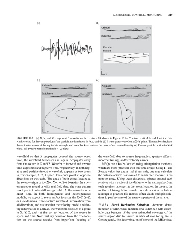
FIGURE 10.9 (a) X, Y, and Z component P waveforms for receiver R4 shown in Figure 10.8a. The two vertical bars delimit the data
window used for the computation of the particle motion shown in (b, c, and d). (b) P wave particle motion in X–Y plane. The numbers indicate
the estimated values of the ray incidence angle and event back‐azimuth at the point of maximum linearity. (c) P wave particle motion in X–Z
plane. (d) P wave particle motion in Y–Z plane.

wavefield so that it propagates beyond the source onset the wavefield due to source frequencies, aperture affects,
time, the wavefield defocuses and, again, propagates away incorrect timing, and/or velocity errors.
from the source in X and Z. We refer to forward and reverse MEQs can also be located using triangulation methods,
time as positive and negative time, respectively. In both neg­ which are more practical with multiple arrays. Using P‐ and
ative and positive time, the wavefield appears as two cones S‐wave velocities and arrival times only, one may calculate
in, for example, X, Z, t space. The cones point in opposite the distance a wave has traveled to reach each receiver in the
directions on the t axis. The apex of both cones located at monitor array. Using these distances, spheres around each
the source origin in the X–t, Y–t, or Z–t domains. In a het­ receiver with a radius of the distance to the earthquake from
erogeneous model or with real field data, the cone pattern each receiver intersect at the event location. In theory, the
is not perfect but is still recognizable. At the correct source method of triangulation should provide a unique solution,
onset time, in both homogenous and heterogeneous although in practice this method often yields multiple solu­
models, we expect to see a perfect focus in the X−Y, X–Z, tions in part because of the narrow aperture of the arrays.
or Y–Z domains. If we capture wavefield information from
all directions, and assume that the velocity model and tim­ 10.4.1.4 Focal Mechanism Solutions Accurate deter­
ing information is correct, the wavefield focuses to a point mination of MEQ focal mechanisms is difficult with down­
in X, Y, Z, and t at the correct location of the source in hole data because of the poor azimuthal coverage of the
space and time. Note that any deviation from the true loca­ source region due to limited number of monitoring wells.
tion of the source results from imperfect focusing of Consequently, the determination of some of the MEQ focal