Page 247 - Fundamentals of Gas Shale Reservoirs

MONITORING PASSIVE SEISMIC EMISSIONS WITH SURFACE AND SHALLOW BURIED ARRAYS 227
120

100
Density (sensors per sq.mi)
80 Aperture area (sq.mi)
Sensors per aperture
Number 60

40

20

0
0 2,000 4,000 6,000 8,000 10,000 12,000
Depth (ft)
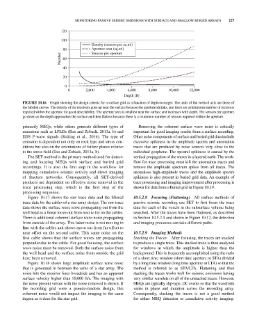
FIGURE 10.16 Graph showing the design criteria for a surface grid as a function of depth‐to‐target. The units of the vertical axis are those of
the labeled curves. The density of the receivers goes up near the surface because the aperture shrinks, and there are a minimum number of receivers
required within the aperture for good detectability. The aperture area is smallest near the surface and increases with depth. The sensors per aperture
go down as the depth approaches the surface and then flattens because there is a minimum number of sensors required within the aperture.

primarily MEQs, while others generate different types of Removing the coherent surface wave noise is critically
emissions such as LPLDs (Das and Zoback, 2013a, b) and important for good imaging results from a surface recording.
EDS P‐wave signals (Sicking et al., 2014). The type of Other noise components of surface and buried grid data include
emission is dependent not only on rock type and stress con­ excessive spikiness in the amplitude spectra and anomalous
ditions but also on the orientations of failure planes relative traces that are produced by noise sources very close to the
to the stress field (Das and Zoback, 2013a, b). individual geophone. The spectral spikiness is caused by the
The SET method is the primary method used for detect­ vertical propagation of the waves in a layered earth. The work­
ing and locating MEQs with surface and buried grid flow for trace processing must kill the anomalous traces and
recordings. It is also the first step in the workflow for remove the amplitude spectrum spikes from all traces. The
mapping cumulative seismic activity and direct imaging anomalous high‐amplitude traces and the amplitude spectra
of fracture networks. Consequently, all SET‐derived spikiness is also present in buried grid data. An example of
products are dependent on effective noise removal in the trace processing and imaging improvement after processing is
trace processing step, which is the first step of the shown for data from a buried grid in Figure 10.19.
processing sequence.
Figure 10.17 shows the raw trace data and the filtered 10.5.2.8 Focusing (Flattening) All surface methods of
trace data for the cables of a star array design. The raw trace passive seismic recording use SET to first focus the trace
data shows the surface wave noise propagating out from the data for each of the voxels in the subsurface volume being
well head as a linear move out from near to far on the cables. searched. After the traces have been flattened, as described
There is additional coherent surface wave noise propagating in Section 10.5.2.1 and shown in Figure 10.12, the detection
from outside of the array. This latter noise is not moving in and imaging processes can take different paths.
line with the cables and shows move out from far offset to
near offset on the second cable. This same noise on the 10.5.2.9 Imaging Methods
first cable shows that the surface waves are propagating Stacking the Traces After focusing, the traces are stacked
perpendicular to the cable. For good focusing, the surface to produce a single trace. This stacked trace is then analyzed
wave noise must be removed. Both the surface noise from for windows in which the amplitude is higher than the
the well head and the surface noise from outside the grid background. This is frequently accomplished using the ratio
have been removed. of a short time window (short time aperture or STA) divided
Figure 10.18 shows large amplitude surface wave noise by a long time window (long time aperture or LTA) so that the
that is generated in between the arms of a star array. The method is referred to as STA/LTA. Flattening and then
noise hits the receiver lines broadside and has an apparent stacking the traces works well for seismic emissions having
surface velocity higher than 10,000 ft/s. The imaging with very similar wavelets on all of the unstacked traces. However,
the noise present versus with the noise removed is shown. If MEQs are typically slip‐type, DC events so that the waveform
the recording grid were a pseudo‐random design, this varies in phase and duration across the recording array.
coherent noise would not impact the imaging to the same Consequently, stacking the traces is not a good method
degree as it does for the star grid. for either MEQ detection or cumulative activity imaging.