Page 245 - Fundamentals of Gas Shale Reservoirs

MONITORING PASSIVE SEISMIC EMISSIONS WITH SURFACE AND SHALLOW BURIED ARRAYS 225
10.5.2.3 Initial Velocity Model The velocity model shot location is a measure of the vertical velocity error
must be accurate in order to obtain correct location of and the error in the X, Y location is a measure of the
MEQs, cumulative activity volumes, and fracture images. lateral velocity gradient. By interactively focusing the
Often, a 1D P‐wave velocity model is constructed from a perf shot and changing the velocity model, the focused
nearby sonic log and the focusing is computed using a 1D location of the perf shot can be moved to match the known
velocity model. This works very well for the small area location of the perf shot in X, Y, and Z. When the focused
around the well being treated for focusing the emissions, location of the perf shot matches the known location of
especially if the strata are horizontal and relatively homo­ the perf shot, the velocity model is correct. Unlike perf
geneous. When there is a lateral velocity gradient in the shots that are located only on the wellbore, MEQs occur
velocity model, the location accuracy can be degraded. throughout the study volume and, therefore, provide an
However, if the magnitude of the velocity gradient is additional constraint on the velocity model. Although the
known then beam steering methods can be used in SET to absolute location of an MEQ is not known independently,
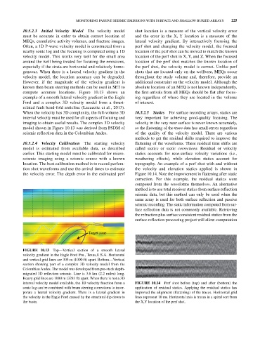
compute accurate locations. Figure 10.13 shows an the first arrivals from all MEQs should be flat after focus­
example of a smooth lateral velocity gradient in the Eagle ing regardless of where they are located in the volume
Ford and a complex 3D velocity model from a thrust‐ of interest.
related fault bend‐fold anticline (Lacazette et al., 2013).
When the velocity has 3D complexity, the full‐volume 3D 10.5.2.5 Statics For surface recording arrays, statics are
interval velocity must be used for all aspects of focusing and very important for achieving good‐quality focusing. The
imaging to obtain useful results. The complex 3D velocity velocity in the very near surface is never known accurately,
model shown in Figure 10.13 was derived from PSDM of so the flattening of the trace data has small errors regardless
seismic reflection data in the Colombian Andes. of the quality of the velocity model. There are various
methods to get the residual shifts required to improve the
10.5.2.4 Velocity Calibration The starting velocity flattening of the waveforms. These residual time shifts are
model is estimated from available data, as described called statics or static corrections. Residual or velocity
earlier. This starting model must be calibrated for micro­ statics accounts for near‐surface velocity variations (i.e.,
seismic imaging using a seismic source with a known weathering effects), while elevation statics account for
location. The best calibration method is to record perfora­ topography. An example of a perf shot with and without
tion shot waveforms and use the arrival times to estimate the velocity and elevation statics applied is shown in
the velocity error. The depth error in the estimated perf Figure 10.14. Note the improvement in flattening after static
correction. For this example, the residual statics were
computed from the waveforms themselves. An alternative
method is to use total receiver statics from surface reflection
seismic data, but this method can only be used when the
same array is used for both surface reflection and passive
seismic recording. The static information computed from sur­
face reflection data is not commonly available. Retrieving
the refraction plus surface consistent residual statics from the

surface reflection processing project will allow computation

Target zone

FIGURE 10.13 Top—Vertical section of a smooth lateral
velocity gradient in the Eagle Ford Fm., Texas,U.S.A. Horizontal
and vertical grid lines are 305 m (1000 ft) apart. Bottom—Vertical
section showing part of a complex 3D velocity model from the
Colombian Andes. The model was developed from pre‐stack depth‐
migrated 3D reflection seismic. Line is 3.6 km (2.2 miles) long.
Heavy grid lines are 1000 m (3281 ft) apart. When there is not a 3D
interval velocity model available, the 1D velocity function from a FIGURE 10.14 Perf shot before (top) and after (bottom) the
sonic log can be combined with beam steering corrections to incor­ application of residual statics. Applying the residual statics has
porate a lateral velocity gradient. There is a lateral gradient in improved the alignment (flattening) of the traces. Horizontal grid
the velocity in the Eagle Ford caused by the structural dip down to lines represent 10 ms. Horizontal axis is traces in a spiral sort from
the basin. the X,Y location of the perf shot.