Page 251 - Fundamentals of Gas Shale Reservoirs

MONITORING PASSIVE SEISMIC EMISSIONS WITH SURFACE AND SHALLOW BURIED ARRAYS 231

19,050 Positive + Negative Positive –
19,100

19,150
N N

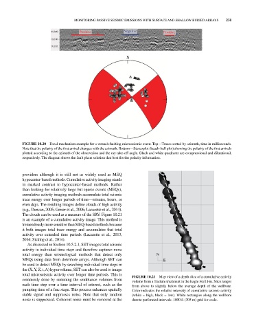
FIGURE 10.20 Focal mechanism example for a wrench‐faulting microseismic event. Top—Traces sorted by azimuth, time in milliseconds.
Note that the polarity of the first arrival changes with the azimuth. Bottom—Stereoplot (beach­ball plot) showing the polarity of the first arrivals
plotted according to the azimuth of the observation and the ray take‐off angle. Black and white quadrants are compressional and dilatational,
respectively. The diagram shows the fault plane solution that best fits the polarity information.

providers although it is still not as widely used as MEQ
hypocenter‐based methods. Cumulative activity imaging stands
in marked contrast to hypocenter‐based methods. Rather
than looking for relatively large but sparse events (MEQs),
cumulative activity imaging methods accumulate total seismic
trace energy over longer periods of time— minutes, hours, or
even days. The resulting images define clouds of high activity
(e.g., Duncan, 2005; Geiser et al., 2006; Lacazette et al., 2014).
The clouds can be used as a measure of the SRV. Figure 10.21
is an example of a cumulative activity image. This method is
tremendously more sensitive than MEQ‐based methods because
it both images total trace energy and accumulates that total
activity over extended time periods (Lacazette et al., 2013,
2014; Sicking et al., 2014).
As discussed in Section 10.5.2.1, SET images total seismic
activity in individual time steps and therefore captures more
total energy than seismological methods that detect only N
MEQs using data from downhole arrays. Although SET can E
be used to detect MEQs by searching individual time steps in
the (X, Y, Z, t, A) hypervolume, SET can also be used to image
total microseismic activity over longer time periods. This is FIGURE 10.21 Map view of a depth slice of a cumulative activity
commonly done by summing the semblance volumes from volume from a fracture treatment in the Eagle Ford Fm. Slice ranges
each time step over a time interval of interest, such as the from above to slightly below the average depth of the wellbore.
pumping time of a frac stage. This process enhances spatially Color indicates the relative intensity of cumulative seismic activity
stable signal and suppresses noise. Note that only random (white = high, black = low). White rectangles along the wellbore
noise is suppressed. Coherent noise must be removed at the denote perforated intervals. 1000 ft (305 m) grid for scale.