
Page 336 - Fundamentals of Gas Shale Reservoirs
P. 336
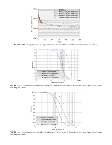
1.E+06
                                                                  Field data
                                                                  Simulated by UGRAS (P10)
                                                                  Simulated by UGRAS (mean)
                                                                  Simulated by UGRAS (P50)
                                    Production (Mcf/month)  1.E+04
                                                                  Simulated by UGRAS (P90)
                                     1.E+05


                                     1.E+03
                                          0      50      100    150     200    250     300
                                                               Month
                FIGURE 14.19  Average production of 476 gas wells in the Haynesville Shale overlaid the mean TRR simulated by UGRAS.

                                      100
                                       90
                                       80
                                       70
                                       60
                                     Percentile  50

                                       40
                                       30
                                               Marcellus (Pearson5)
                                       20      Eagle Ford (Loglogistic)
                                       10      Barnett (Loglogistic)
                                               Haynesville (Lognormal)
                                       0
                                        1              10             100            1000
                                                         OGIP (Bcf/section)
            FIGURE 14.20  Comparison between probabilistic distributions of OGIP per section for four shale gas plays in the United States (Adapted
            from Dong et al., 2014).

                                    100

                                     90
                                     80
                                     70

                                     60
                                    Percentile  50

                                     40
                                     30
                                             Barnett (lognormal)
                                     20      Eagle Ford (invGauss)
                                     10      Marcellus (invGauss)
                                             Haynesville (lognormal)
                                      0
                                       1                     10                   100
                                                          TRR (Bcf/section)
            FIGURE 14.21  Comparison between probabilistic distributions of TRR per section for four shale gas plays in the United States (Adapted
            from Dong et al., 2014).