
Page 288 - Fundamentals of Reservoir Engineering
P. 288
OILWELL TESTING 225
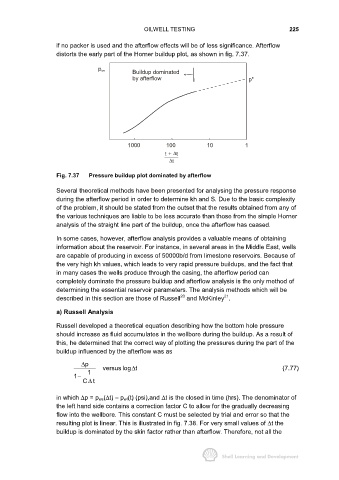
if no packer is used and the afterflow effects will be of less significance. Afterflow
distorts the early part of the Horner buildup plot, as shown in fig. 7.37.
p ws
Buildup dominated
by afterflow p*
1000 100 10 1
t +∆ t
t ∆
Fig. 7.37 Pressure buildup plot dominated by afterflow
Several theoretical methods have been presented for analysing the pressure response
during the afterflow period in order to determine kh and S. Due to the basic complexity
of the problem, it should be stated from the outset that the results obtained from any of
the various techniques are liable to be less accurate than those from the simple Horner
analysis of the straight line part of the buildup, once the afterflow has ceased.
In some cases, however, afterflow analysis provides a valuable means of obtaining
information about the reservoir. For instance, in several areas in the Middle East, wells
are capable of producing in excess of 50000b/d from limestone reservoirs. Because of
the very high kh values, which leads to very rapid pressure buildups, and the fact that
in many cases the wells produce through the casing, the afterflow period can
completely dominate the pressure buildup and afterflow analysis is the only method of
determining the essential reservoir parameters. The analysis methods which will be
20
21
described in this section are those of Russell and McKinley .
a) Russell Analysis
Russell developed a theoretical equation describing how the bottom hole pressure
should increase as fluid accumulates in the wellbore during the buildup. As a result of
this, he determined that the correct way of plotting the pressures during the part of the
buildup influenced by the afterflow was as
∆ p
versus log t ∆ (7.77)
1
1−
Ct
∆
in which ∆p = p ws(∆t) − p wf(t) (psi),and ∆t is the closed in time (hrs). The denominator of
the left hand side contains a correction factor C to allow for the gradually decreasing
flow into the wellbore. This constant C must be selected by trial and error so that the
resulting plot is linear. This is illustrated in fig. 7.38. For very small values of ∆t the
buildup is dominated by the skin factor rather than afterflow. Therefore, not all the