Page 289 - Fundamentals of Reservoir Engineering
P. 289

OILWELL TESTING                                    226

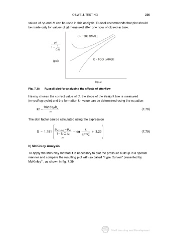
                     values of ∆p and ∆t can be used in this analysis. Russell recommends that plot should
                     be made only for values of ∆t measured after one hour of closed-in time.


                                                       C - TOO SMALL

                                       p∆
                                         1
                                     1 −
                                        C∆t


                                                                  C - TOO LARGE
                                      (psi)


                                                                    log ∆t

                     Fig. 7.38  Russell plot for analysing the effects of afterflow

                     Having chosen the correct value of C. the slope of the straight line is measured
                     (m−psi/log cycle) and the formation kh value can be determined using the equation

                               162.6q B
                                      µ
                           kh =          o                                                          (7.78)
                                    m
                     The skin factor can be calculated using the expression


                                        p     − p           k
                                           −
                           S =  1.151    wf(1 hr)  wf  − log   2  +  3.23                           (7.79)
                                          −
                                           11/ C t ∆      φµ cr w
                                            m

                     b) McKinley Analysis

                     To apply the McKinley method it is necessary to plot the pressure buildup in a special
                     manner and compare the resulting plot with so called "Type Curves" presented by
                              21
                     McKinley , as shown in fig. 7.39.
   284   285   286   287   288   289   290   291   292   293   294