Page 290 - Fundamentals of Reservoir Engineering

OILWELL TESTING 227

T T
t ∆ t ∆ = 10 000 F = 5 000
(mins) (mins) F
T
1000 1000 F = 2 500

100 100

(a) (b)
10 10

1 1
1 10 100 1000 10 -4 10 -3 10 -2 10 -1
∆p (psi) ∆pF
q

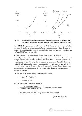
Fig. 7.39 (a) Pressure buildup plot on transparent paper for overlay on (b) McKinley
type curves, derived by computer solution of the complex afterflow problem

A set of McKinley type curves is included as fig. 7.40. These curves were computed by
numerical simulation of the complex afterflow process by forming a dynamic balance
between the capacity of the wellbore to store fluid and the resistance of the wellbore to
the flow of fluid from the reservoir.

-7
2
All the curves were computed for a constant value of φµ cr /k = 1.028×10 cp.
w
sq ft/(mD psi), since in his original paper McKinley has demonstrated that the shape of
the type curves is insensitive to variation in the value of this parameter. Furthermore,
the curves were computed assuming no mechanical skin factor. If a well is damaged
this fact is evident since the pressure buildup plot will deviate from the McKinley type
curve and while the analysis does not explicitly determine the skin factor, it does allow
a comparison to be made between the kh values in the damaged and undamaged
parts of the reservoir.

The abscissa of fig. 7.40 is for the parameter ∆pF/q where

∆p= p ws (∆t) – p wf (t) (psi)

q = oil rate in rb/d

and F is the so called "wellbore parameter"

Wellbore area (sq.ft)
F = (for partially liquid filled wells)
Wellbore liquid gradient (psi/ ft)

3
1
−
F = Wellbore fluid compressibility (psi ) Wellbore volume (ft )
×
(for fluid filled wells)