Page 150 - Fundamentals of Water Treatment Unit Processes : Physical, Chemical, and Biological

Sedimentation 105

1.0 Conclusions from Camp’s ideal settling theory applicable
P o =0.94
to practice are
0.9
Integral 1. The term ‘‘overflow velocity,’’ sometimes called
area
0.8
‘‘surface overflow rate’’ (SOR), has been established
in the vernacular in practice and as a way of thinking
0.7 about settling basins.
2. The fraction of a suspension removed is a function
0.6 of the ‘‘overflow velocity,’’ v o . Since, v o ¼ Q=A
(plan), the plan area of the basin is the focus.
P 0.5
3. Depth, and by corollary detention time, has no role in
the removal of a discrete particle suspension.
0.4
4. The settling path of a particle having fall velocity v s
is a straight line from its position at the inlet end of
0.3 the settling zone. The iso-concentration lines for a
v o =0.11 cm/s of the basin.
0.2 given suspension are straight lines from the inlet end

0.1 5. Long narrow basins can minimize the effects of short
circuiting.
0.0
For flocculent suspensions, removal depends upon both over-
0.0000 0.0005 0.0010 0.0015 0.0020
flow velocity and detention time. This is the topic of Section 6.5.
v (m/s)
s
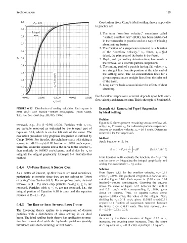
FIGURE 6.12 Distribution of settling velocities. Each square is Example 6.4 Removal of Type I Suspension
(0.01 cm=s) 0.05 fraction ¼ 0.0005 cm=s=square. (From Camp, by Ideal Settling
T.R., Am. Soc. Civil Eng., III, 895, 1946.)
Problem
Figure 6.12 shows percent remaining versus overflow vel-
removed, e.g., R ¼ (1 0.94) ¼ 0.06. Particles with v s < v o
ocity, i.e., P versus v o , for a discrete particle suspension.
are partially removed as indicated by the integral part of Assume an overflow velocity, v o ¼ 0.11 cm=s. Determine
Equation 6.18, which is on the left side of the curve. The removal R for the suspension.
evaluation procedure is by graphical integration as outlined by
Method
Camp (1946). For the plot, the technique starts with sizing a
Apply Equation 6.18, i.e.
square, i.e., (0.01 cm=s) 0.05 fraction ¼ 0.0005 cm=s square;
therefore, count the squares above the curve to the desired v o , 1 ð
then multiply by 0.0005 cm=s=square, and divide by v o to R ¼ (1 P o ) þ v s dP (Ex6:4:1)(6:18)
v o
integrate the integral graphically. Example 6.4 illustrates this
method. From Equation 6.18, evaluate the function, R ¼ f(v o ). This
can be done by integrating the integral graphically and
adding the associated (1 P o ) value.
6.4.4 UP-FLOW BASINS:ASPECIAL CASE
Solution
As a matter of interest, up-flow basins are used sometimes, From Figure 6.12, for the overflow velocity, v o ¼ 0.11
particularly as retrofits since they are not subject to ‘‘short cm=s, P o ¼ 0.94. The graphical integration is done as indi-
cated in Figure 6.10b. Each square is: [0.01 cm=s 0.05
circuiting’’ (see Section 6.8.1). For an up-flow basin, the total
fraction] ¼ 0.0005 cm=s=square. Counting the squares
removal is (1 P o ) since only particles having v s v o are
above the curve of Figure 6.12 between the limits 0
removed. Particles with v s v o are not removed, i.e., the
and 0.11 cm=s, with corresponding P o ¼ 0.84, gives
integral portion of Equation 6.18 is zero, and the equation
about 73 squares. Thus, 73 squares 0.0005 cm=s=
reduces to R ¼ (1 P o ).
square ¼ 0.0365 cm=s, the value of the integral. Next,
dividing by v o ¼ 0.11 cm=s, gives, (0.0365 cm=s)=(0.11
cm=s) ¼ 0.33 fraction of suspension removed between
6.4.5 THE ROLE OF IDEAL SETTLING BASIN THEORY
the limits, 0 < v s < 0.11 cm=s. The total removal, R ¼
The foregoing theory applies to a suspension of discrete (1 0.94) þ 0.33 ¼ 0.39.
particles with a distribution of sizes settling in an ideal Comment
basin. The ideal settling basin theory has application to prac-
As seen by the flatter curvature of Figure 6.12 as v o
tice but cannot deal with the hydraulic problems (mainly increases, the counting error increases. Thus, the count
turbulence and short circuiting) of real basins. of 73 squares for v o ¼ 0.11 cm=s is perhaps 1 square.