Page 148 - Fundamentals of Water Treatment Unit Processes : Physical, Chemical, and Biological

Sedimentation 103

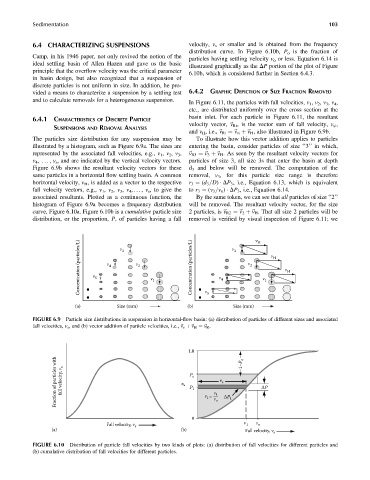
6.4 CHARACTERIZING SUSPENSIONS velocity, v s or smaller and is obtained from the frequency
distribution curve. In Figure 6.10b, P o is the fraction of
Camp, in his 1946 paper, not only revived the notion of the
particles having settling velocity v o or less. Equation 6.14 is
ideal settling basin of Allen Hazen and gave us the basic
illustrated graphically as the DP portion of the plot of Figure
principle that the overflow velocity was the critical parameter
6.10b, which is considered further in Section 6.4.3.
in basin design, but also recognized that a suspension of
discrete particles is not uniform in size. In addition, he pro-
vided a means to characterize a suspension by a settling test 6.4.2 GRAPHIC DEPICTION OF SIZE FRACTION REMOVED
and to calculate removals for a heterogeneous suspension.
In Figure 6.11, the particles with fall velocities, v 1 , v 2 , v 3 , v 4 ,
etc., are distributed uniformly over the cross section at the
basin inlet. For each particle in Figure 6.11, the resultant
6.4.1 CHARACTERISTICS OF DISCRETE PARTICLE
velocity vector, ~ v Ri , is the vector sum of fall velocity, v si ,
SUSPENSIONS AND REMOVAL ANALYSIS
and v H , i.e., ~ v Ri ¼~ v si þ~ v H , also illustrated in Figure 6.9b.
The particles size distribution for any suspension may be To illustrate how this vector addition applies to particles
illustrated by a histogram, such as Figure 6.9a. The sizes are entering the basin, consider particles of size ‘‘3’’ in which,
represented by the associated fall velocities, e.g., v 1 , v 2 , v 3 , ~ v R3 ¼~ v 3 þ~ v H . As seen by the resultant velocity vectors for
v 4 , ... , v s , and are indicated by the vertical velocity vectors. particles of size 3, all size 3s that enter the basin at depth
Figure 6.9b shows the resultant velocity vectors for these d 3 and below will be removed. The computation of the
same particles in a horizontal flow settling basin. A common removal, v 3 , for this particle size range is therefore
=
horizontal velocity, v H , is added as a vector to the respective r 3 ¼ (d 3 D) DP 3 , i.e., Equation 6.13, which is equivalent
=
fall velocity vectors, e.g., v 1 , v 2 , v 3 , v 4 ,. .., v s , to give the to r 3 ¼ (v 3 v o ) DP 3 , i.e., Equation 6.14.
associated resultants. Plotted as a continuous function, the By the same token, we can see that all particles of size ‘‘2’’
histogram of Figure 6.9a becomes a frequency distribution will be removed. The resultant velocity vector, for the size
curve, Figure 6.10a. Figure 6.10b is a cumulative particle size 2 particles, is ~ v R2 ¼~ v 2 þ~ v H . That all size 2 particles will be
distribution, or the proportion, P, of particles having a fall removed is verified by visual inspection of Figure 6.11; we

v
Concentration (particles/L) v 5 v 4 v 3 v 2 v 1 Concentration (particles/L) v 4 v 3 v 2 v 1 v H v H
H

(a) Size (mm) (b) v 5 Size (mm)

FIGURE 6.9 Particle size distributions in suspension in horizontal-flow basin: (a) distribution of particles of different sizes and associated
fall velocities, v s , and (b) vector addition of particle velocities, i.e., ~ v s þ~ v H ¼~ v R .

1.0 1–P o
Fraction of particles with fall velocity, v s P P o 1 r = v 1 v s ΔP 1 ΔP

P
1

0 v o
Fall velocity, v s v 1 v o
(a) (b)
Fall velocity, v s
FIGURE 6.10 Distribution of particle fall velocities by two kinds of plots: (a) distribution of fall velocities for different particles and
(b) cumulative distribution of fall velocities for different particles.