Page 158 - Fundamentals of Water Treatment Unit Processes : Physical, Chemical, and Biological

Sedimentation 113

may be depicted by CFD, see Box 6.1, which is based upon 6.7.3 DISPERSION TESTS USING A TRACER
hydraulic theory and executed by computer simulation.
The traditional means to assess the hydraulic characteristics of
Review of these topics helps to understand behavior of
a basin is to perform a dye dispersion test (Camp, 1946). To
real settling basins, albeit it does not permit predictions
conduct the test, a ‘‘tracer’’ is injected in the influent flow; its
of performance.
concentration in the basin effluent is then measured with time.
A suitable tracer may be any substance that does not react or
6.7.1 FLOW PATTERNS AND SHORT CIRCUITING degrade and that may be detected at low concentrations. Such
tracers include Rhodamine WT a fluorescent dye (which is
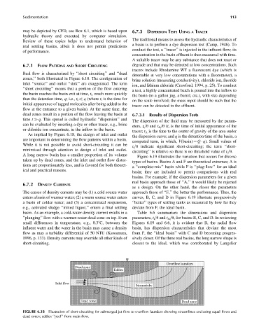
Real flow is characterized by ‘‘short circuiting’’ and ‘‘dead
detectable at very low concentrations with a fluorometer), a
zones,’’ both illustrated in Figure 6.18. The configuration of
brine solution (measuring conductivity), chloride ion, fluoride
inlet ‘‘source’’ and outlet ‘‘sink’’ are exaggerated. The term
ion, and lithium chloride (Crawford, 1994, p. 25). To conduct
‘‘short circuiting’’ means that a portion of the flow entering
a test, a highly concentrated batch is poured into the inflow to
the basin reaches the basin exit at time, t i , much more quickly
the basin (in a gallon jug, a barrel, etc.), with size depending
than the detention time, q; i.e., t i q (where t i is the time for
on the scale involved; the mass input should be such that the
initial appearance of tagged molecules after being added to the
tracer can be detected in the effluent.
flow at the entrance to a given basin). At the same time, the
dead zones result in a portion of the flow leaving the basin at 6.7.3.1 Results of Dispersion Tests
time t q. This spread is called hydraulic ‘‘dispersion’’ and
The dispersion of the fluid may be measured by the param-
can be evaluated by inserting a dye or other tracer, e.g., brine
eters, t i =u and t A =u (t i is the time of initial appearance of the
or chloride ion concentrate, in the inflow to the basin.
tracer; t A is the time to the center of gravity of the area under
As implied by Figure 6.18, the design of inlet and outlet
the dispersion curve; and q is the detention time of the basin, a
are important in determining the flow patterns within a basin.
computed term, in which, V(basin) ¼ Q q). Small values of
While it is not possible to avoid short-circuiting it can be
t i =u indicate significant short-circuiting; the term ‘‘short-
minimized through attention to design of inlet and outlet.
circuiting’’ is relative so there is no threshold value of t i =u.
A long narrow basin has a smaller proportion of its volume
Figure 6.19 illustrates the variation that occurs for diverse
taken up by dead zones, and the inlet and outlet flow distor-
types of basins. Basins A and F are theoretical extremes; A is
tions are proportionately less, and is favored for both theoret-
a ‘‘complete-mix’’ basin while F is ‘‘plug-flow’’ for an ideal
ical and practical reasons.
basin; they are included to permit comparisons with real
basins. For example, if the dispersion parameters for a given
real basin approach those of ‘‘A,’’ it would likely be rejected
6.7.2 DENSITY CURRENTS
as a design. On the other hand, the closer the parameters
The causes of density currents may be (1) a cold source water approach those of ‘‘F,’’ the better the performance. Thus, the
enters a basin of warmer water; (2) a warm source water enters curves, B, C, and D in Figure 6.19 illustrate progressively
a basin of colder water; and (3) a concentrated suspension, ‘‘better’’ types of settling tanks as measured by how far they
e.g., activated sludge ‘‘mixed liquor,’’ enters a final settling deviate from F, the ideal basin.
basin. As an example, a cold-water density current results in a Table 6.6 summarizes the dimensions and dispersion
‘‘plunging’’ flow with a warmer-water dead zone on top. Even parameters, t i =u and t A =u, for basins B, C, and D. In reviewing
small differences in temperature, e.g., 0.38C, between the Figures 6.19 and 6.6, it is evident that B, the radial flow
influent water and the water in the basin may cause a density basin, has dispersion characteristics that deviate the most
flow as may a turbidity differential of 50 NTU (Kawamura, from F, the ‘‘ideal basin’’ with C and D becoming progres-
1996, p. 133). Density currents may override all other kinds of sively closer. Of the three real basins, the long narrow shape is
short-circuiting. closest to the ideal, which was corroborated by Langelier

Overflow launders
Dead zone
Eddies

Inlet flow
Streamtube

Dead zone Dead zone

FIGURE 6.18 Illustration of short-circuiting for submerged jet flow to overflow launders showing streamlines enclosing equal flows and
dead zones; eddies ‘‘peel’’ from main flow.