Page 289 - Fundamentals of Water Treatment Unit Processes : Physical, Chemical, and Biological

244 Fundamentals of Water Treatment Unit Processes: Physical, Chemical, and Biological

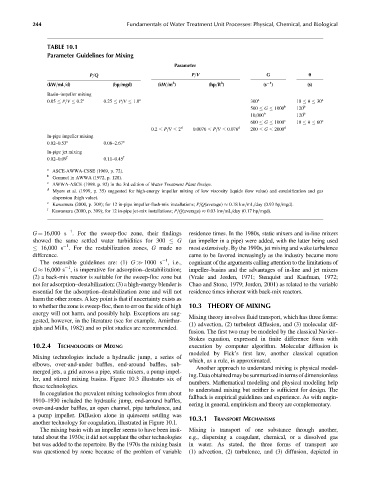
TABLE 10.1
Parameter Guidelines for Mixing
Parameter
P=Q P=V G u
3
1
3
(kW=mL=d) (hp=mgd) (kW=m ) (hp=ft ) (s ) (s)
Basin–impeller mixing
a a a a
0.05 P=V 0.2 0.25 P=V 1.0 300 10 u 30
500 G 1000 b 120 b
10,000 b 120 b
600 G 1000 c 10 u 60 c
0.2 P=V 2 d 0.0076 P=V 0.076 d 200 G 2000 d
In-pipe impeller mixing
0.02–0.53 e 0.08–2.67 e
In-pipe jet mixing
0.02–0.09 f 0.11–0.45 f
a
ASCE-AWWA-CSSE (1969, p. 72).
b
Gemmel in AWWA (1972, p. 128).
c
AWWA-ASCE (1998. p. 92) in the 3rd edition of Water Treatment Plant Design.
d
Myers et al. (1999, p. 35) suggested for high-energy impeller mixing of low viscosity liquids (low value) and emulsification and gas
dispersion (high value).
e
Kawamura (2000, p. 309); for 12 in-pipe impeller-flash-mix installations; P=Q(average) 0.18 kw=mL=day (0.93 hp=mgd).
f
Kawamura (2000, p. 309); for 12 in-pipe jet-mix installations; P=Q(average) 0.03 kw=mL=day (0.17 hp=mgd).
1
G ¼ 16,000 s . For the sweep-floc zone, their findings residence times. In the 1980s, static mixers and in-line mixers
showed the same settled water turbidities for 300 G (an impeller in a pipe) were added, with the latter being used
1
16,000 s . For the restabilization zones, G made no most extensively. By the 1990s, jet mixing and wake turbulence
difference. came to be favored increasingly as the industry became more
1
The ostensible guidelines are: (1) G >> 1000 s , i.e., cognizant of the arguments calling attention to the limitations of
1
G 16,000 s , is imperative for adsorption–destabilization; impeller–basins and the advantages of in-line and jet mixers
(2) a back-mix reactor is suitable for the sweep-floc zone but (Vrale and Jorden, 1971; Stenquist and Kaufman, 1972;
not for adsorption–destabilization; (3) a high-energy blender is Chao and Stone, 1979; Jorden, 2001) as related to the variable
essential for the adsorption–destabilization zone and will not residence times inherent with back-mix reactors.
harm the other zones. A key point is that if uncertainty exists as
to whether the zone is sweep-floc, then to err on the side of high 10.3 THEORY OF MIXING
energy will not harm, and possibly help. Exceptions are sug-
Mixing theory involves fluid transport, which has three forms:
gested, however, in the literature (see for example, Amirthar-
(1) advection, (2) turbulent diffusion, and (3) molecular dif-
ajah and Mills, 1982) and so pilot studies are recommended.
fusion. The first two may be modeled by the classical Navier–
Stokes equation, expressed in finite difference form with
10.2.4 TECHNOLOGIES OF MIXING execution by computer algorithm. Molecular diffusion is
modeled by Fick’s first law, another classical equation
Mixing technologies include a hydraulic jump, a series of
which, as a rule, is approximated.
elbows, over-and-under baffles, end-around baffles, sub-
Another approach to understand mixing is physical model-
merged jets, a grid across a pipe, static mixers, a pump impel-
ing.Dataobtainedmaybesummarizedintermsofdimensionless
ler, and stirred mixing basins. Figure 10.3 illustrates six of
numbers. Mathematical modeling and physical modeling help
these technologies.
to understand mixing but neither is sufficient for design. The
In coagulation the prevalent mixing technologies from about
fallback is empirical guidelines and experience. As with engin-
1910–1930 included the hydraulic jump, end-around baffles,
eering in general, empiricism and theory are complementary.
over-and-under baffles, anopenchannel,pipeturbulence, and
a pump impeller. Diffusion alone in quiescent settling was
10.3.1 TRANSPORT MECHANISMS
another technology for coagulation, illustrated in Figure 10.1.
The mixing basin with an impeller seems to have been insti- Mixing is transport of one substance through another,
tuted about the 1930s; it did not supplant the other technologies e.g., dispersing a coagulant, chemical, or a dissolved gas
but was added to the repertoire. By the 1970s the mixing basin in water. As stated, the three forms of transport are
was questioned by some because of the problem of variable (1) advection, (2) turbulence, and (3) diffusion, depicted in