Page 536 - Fundamentals of Water Treatment Unit Processes : Physical, Chemical, and Biological

Adsorption 491

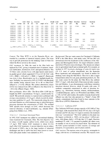
v v v wf Q Q Q
wf
wf
(sat)
L L L(sat) t(run) L L L wf L L L(reactor) A(total) n(col) D D (bed) V(bed) M M (carbon) Unit Cost $(carbon)
t
(sat)
(bed)
(bed)
V V
M(carbon)
(bed)
t
n
A A
(col)
(total)
(total)
n
D(bed)
(run)
(run)
(col)
(reactor)
(reactor)
Unit
Unit Cost
Cost
$(carbon)
$(carbon)
(carbon)
wf
wf
3 3 3
3 3 3
(m)
(m)
=
day)
day)
(d)
C)
(d)
kg
kg
=
(m
($ ($
(m
(m
=
=
(m)
(m
(m)
(m
=
(m
(mgd)
(mgd)
(m )
(m
s)
=
s)
(m
($)
C)
($)
(m)
(m)
(#)
(m)
(#)
A(col)
A(col)
=
h)
h)
=
(m
(m
(kg)
(kg)
(m=h) (m=day) (m) (d) (m) (m ) ) (mgd) (m =s) (m 2 2 2 ) ) (#) A(col) (m) (m ) ) ) (kg) ($=kg C) ($)
10
2.00
10
126,696
25.85
1.00
0.66
284
2.00
0.66
191964
25.85
0.00017 65 0.0042 2 2 10 2360 1.00 11.00 2.00 0.0876 25.85 1.00 25.85 5.74 284 191964 0.66 126,696
126,696
1.00
1.00
25.85
5.74
11.00
2360
11.00
5.74
25.85
0.0001765
2360
0.00017
0.004
0.0876
0.0876
191964
65
0.004
284
1.00
0.004
12.93
2.00
0.004
284
2360
2360
12.93
0.0876
25.85
1.00
1.00
25.85
65
2.00
0.0876
65
0.0001765 0.0042 2 2 10 2360 1.00 11.00 2.00 0.0876 25.85 2.00 12.93 4.06 284
2.00
284
0.00017
10
10
2.00
4.06
4.06
0.00017
11.00
11.00
0.0876
25.85
0.0876
1.00
1.00
2.00
11.00
2.00
0.00017 65 0.004 2 2 10 2360 1.00 11.00 2.00 0.0876 25.85 4.00 6.46 2.87 284
11.00
0.00017
4.00
4.00
0.0001765
0.0042
2360
65
284
284
2360
10
10
2.87
0.004
2.87
6.46
6.46
25.85
4.00
4.00
10
11.00
11.00
0.004
25.85
2.87
2.00
2.00
10
0.0002036
0.00020
0.00020 36 0.004 9 9 10 2047 1.00 11.00 2.00 0.0876 25.85 4.00 6.46 2.87 284
2.87
0.0876
2047
284
36
2047
0.0876
25.85
6.46
0.0049
6.46
284
1.00
1.00
01
2.00
2.00
1.00
0.0096
0.0876
1.00
126,696
0.0876
0.009
126,696
0.66
191964
284
11.00
11.00
25.85
284
25.85
1.00
1.00
1041
1041
25.85
0.66
191964
5.74
25.85
5.74
0.00040 01 0.009 6 6 10 1041 1.00 11.00 2.00 0.0876 25.85 1.00 25.85 5.74 284 191964 0.66 126,696
0.0004001
10
10
0.00040
0.0876
25.85
25.85
284
284
1.00
1.00
943
25.85
20
0.010
5.74
5.74
0.0106
943
10
10
25.85
2.00
0.0876
2.00
1.00
1.00
0.00044
0.0004420
0.00044 20 0.010 6 6 10 943 1.00 11.00 2.00 0.0876 25.85 1.00 25.85 5.74 284
11.00
11.00
284
284
5.74
1.00
1.00
25.85
5.74
25.85
1.00
11.00
653
1.00
11.00
0.0876
0.0876
2.00
2.00
0.0006379
79
0.00063 79 0.0153 3 3 10 653 1.00 11.00 2.00 0.0876 25.85 1.00 25.85 5.74 284
0.00063
0.015
10
653
0.015
10
25.85
25.85
0.172
10
10
0.1727
5.74
5.74
25.85
1.00
1.00
58
58
25.85
191964
191964
284
0.66
126,696
126,696
0.66
0.0071954
25.85
54
0.00719
284
25.85
0.00719 54 0.172 7 7 10 58 1.00 11.00 2.00 0.0876 25.85 1.00 25.85 5.74 284 191964 0.66 126,696
2.00
1.00
0.0876
0.0876
2.00
1.00
11.00
11.00
25.85
25.85
284
284
10
0.0876
10
0.01296
0.0129618
2.00
18
2.00
0.311
0.3111
5.74
0.01296 18 0.311 1 1 10 32 1.00 11.00 2.00 0.0876 25.85 1.00 25.85 5.74 284 244008 0.66 161,045
5.74
161,045
0.66
0.66
244008
25.85
1.00
11.00
1.00
11.00
244008
1.00
25.85
1.00
161,045
0.0876
32
32
Given
n
Given
(col)
(col)
t
Cos
Unit
t
Cost
Cos
Unit
Cost
Q
=
A
Given t ¼ L (sat) = v A A A ¼ Q=HLR A(col) ¼ A(total)=n(col) Given Cost ¼ Unit Cost
Given t ¼ L(sat)=v
Q
A
HLR
HLR
A A
=
(col)
(col)
=
(total
n
(total
=
)
)
Given t ¼ L(sat)=v wf L ¼ L(sat)þL wfwf L ¼ L(sat)þL wfwf L ¼ L(sat)þL wf
¼
¼
¼
¼
¼
¼
* * *
Given
(total)
Estimated
ted
A
Estima
(total)
A
V V
(carbon)
Given
Given
M
v v wf ¼ HLR C o =(X (C o ) r (1 P)¼ HLR C o =(X (C o ) r (1 P)¼ HLR C o =(X (C o ) r (1 P) Estima ted Given Given V(bed) ¼ L(reactor) A(total) M(carbon)
(carbon)
M
(reactor)
(reactor)
(bed)
L
Given
(bed)
L
wf
v wf

¼
¼
(bed)
(bed)
V
V
(app)
r
(app)
r
(carbon)
(carbon)
M M
M(carbon) ¼ V(bed) r(app)
¼
¼

Context: The Nitro WTP is on the Kanawha River, sur- Background: The raw water source for Cincinnati’s California
rounded by a number of chemical industry plants. The issue WTP is the Ohio River, with intake some 745 km (463 mi)
was to provide protection for the drinking water of Nitro for downstream from the headwaters at the confluence of the Alle-
which the River served as the source. gheny and Monongahela Rivers. Six major tributaries contrib-
GAC treatment: In 1966, the sand in the filter beds was uted about 270 point source discharges. The streams are subject
replaced by GAC, giving a treatment train of aeration, chem- also to agricultural runoff and accidental spills. For example, an
ical clarification, disinfection, GAC adsorption=filtration. The incident in 1977 involved a discharge of some 64 metric tons
10 filters were concrete boxes with pipe-lateral under-drains (70 U.S. tons) of carbon tetrachloride into the Kanawha
in graded gravel which supported 0.76 m (2.5 ft) GAC with River (upstream) and subsequently was found in intakes for
2
2.44 HLR 4.88 m=h(1 HLR 2 gpm=ft ). Backwash drinking water along the Ohio River. The river is also a major
was every 4 days. Reactivation was by a multiple-hearth fur- transportation artery for coal, grain, petroleum products, etc. The
nace. Turbidity was removed to 0.05–0.15 NTU with threshold raw water source for the plant, the Ohio River, has ambient
odor number being reduced from 20 to 80 in filter=GAC TOC 3mg=L with about half of that removed after coagula-
influent to 3 in the effluent. The carbon chloroform extract tion and filtration. A gas chromatogram (with flame ionization
(CCE) was reduced from 200 as influent to the filter=GAC to detection) showed, however, about 30 peaks with some 15
<40 in the effluent (Hager, 1969). synthetic compounds enumerated in order of detection fre-
quency, e.g., chloroform, benzene, toluene, dichloromethane,
Micro-pollutants—River Elbe: The River Elbe (1100 km in
1,2-dichlorobenzene, and so on (Westerhoff and Miller, 1986,
length) has DOC concentrations 6mg=L, caused mostly by
p. 148). In GAC pilot studies, the number of peaks found in the
runoff. The pesticide atrazine is a typical micro-pollutant with
effluent was only four (also present in a ‘‘blank’’). Some 200
average concentrations 0.14 mg=L, which exceeds the drink-
organic contaminants had been found in trace amounts in the
ing water guideline 0.1 mg=L. The waterworks along the river
Ohio River (AWWA Mainstream, 1992).
use bank filtration as a first treatment step in which biological
processes decrease the concentration of DOC. The residual
DOC adsorbs more strongly on GAC, which decreases the 15.4.3.3.3 California WTP
3
removal efficiency of micro-pollutants, e.g., atrazine (Fore- The California WTP had a design capacity of 833,000 m =day
going from Müller et al., 1996). (220 mgd), with measured flow about 454 mL=day (120 mgd)
in winter and 503 mL=day (133 mgd) in summer; the treatment
15.4.3.3.2 Cincinnati Municipal Plant train was ‘‘conventional.’’ The GAC addition to the plant was
In 1992, GAC treatment was added to conventional drinking the largest worldwide (c. 2003), serving about 1 million per-
water treatment for Cincinnati, Ohio. The first objective was sons, with Q(max daily) ¼ 470 mL=day (175 mgd). Reactors
to reduce overall organic carbon levels, which were about numbered 12, with 7–11 operated in parallel; the others were
1.5 mg=L TOC before GAC treatment to about 0.2–0.6 on standby or out of service for reactivation. The elements of
mg=L after GAC treatment. A second objective was to reduce the GAC system included (1) GAC reactors, (2) storage and
the hazard of SOCs, due to the large number of industrial transport, (3) regeneration, and (4) plant controls.
discharges and due to spills that have been known to occur. GAC reactors: The reactors were to be gravity, rectangular in
GAC pilot plant studies were initiated in 1977. shape, with the box of reinforced concrete. The reactors were