Page 535 - Fundamentals of Water Treatment Unit Processes : Physical, Chemical, and Biological

Physical,
Processes:
Chemical,
Biological
and
Unit
Fundamentals
Fundamentals of Water Treatment Unit Processes: Physical, Chemical, and Biological
of
Treatment
Water
490
490
490 Fundamentals of Water Treatment Unit Processes: Physical, Chemical, and Biological
TABLE
CD15.8
TABLE CD15.8
TABLE CD15.8
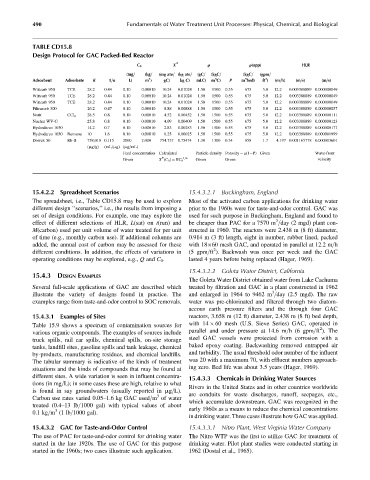
Design Protocol for GAC Packed-Bed Reactor
Proto
Design
Design Proto col for GAC Packe d-Bed Reactor
Packe
Reactor
d-Bed
col
for
GAC
(app)
HLR
X X
C C 0 0 X * * * r r r r(app) HLR
(app)
HLR
C 0
r r
(kgC
(gC=
(mg
(mg
(gC
(kg
(kg
ate
(gpm
(gpm=
(kgC=
(mg ate= (kg ate=
(kgC
(mg
ate
(kg
(mg= = = (kg= = = (mg ate = = (kg ate = = (gC = = (kgC= = = (kgC = = (gpm = =
(kgC
3 3 3
2 2 2
Adsorbat
(m
Adsorbat
m C)
m m
kg
kg C)
m bed)
gC)
gC)
C)
1 1
=
s)
Adsorben
h)
Adsorben t t Adsorbate e e K K K 1=n n n L) L) L) m ) ) ) gC) kg C) mLC ) ) m m 3 3 3 C) P P P m m 3 3 3 bed) ft ft ft ) ) ) ( ( (m=h) (m = = s) (m = = s)
=
s)
(m
(m=s)
h)
mLC
(m=s)
mLC)
bed)
Adsorbent
C)
=
=
m
m
28.2
0.01024
0.01024
Wittcarb
0.000
0.000
Wittcarb 950
0.10
0.10
Wittcarb 950 TCE 28.2 0.44 0.10 0.00010 10.24 0.01024 1.50 1500 0.55 675 5.0 12.2 0.003388889 0.000000049
10.24
10.24
0049
10
0.44
0.44
10
28.2
0.00000
675
675
0.55
0.00000
950
0.55
5.0
0.0033888
89
89
0.0033888
5.0
12.2
12.2
1.50
1500
1500
TCE
1.50
0049
TCE
12.2
5.0
5.0
0.01024
0.01024
0.0033888
0.10
89
0.0033888
89
12.2
0.10
1.50
10
1500
0.55
0.00000
10.24
10.24
0049
1500
0.000
675
1.50
0.00010
0.00000
0.55
675
0049
28.2
TCE
28.2
0.44
0.44
TCE
Wittcarb
Wittcarb 950 TCE 28.2 0.44 0.10 0.000 10 10.24 0.01024 1.50 1500 0.55 675 5.0 12.2 0.003388889 0.000000049
Wittcarb
950
950
12.2
12.2
0.0033888
10.24
5.0
5.0
10.24
89
0.10
0.10
89
0.0033888
10
10
28.2
950
1500
1500
TCE
1.50
1.50
TCE
675
0.01024
0.01024
675
0.55
0.55
28.2
0.44
0.44
0.000
0.000
Wittcarb 950 TCE 28.2 0.44 0.10 0.00010 10.24 0.01024 1.50 1500 0.55 675 5.0 12.2 0.003388889 0.000000049
0.00000
0.00000
Wittcarb 950
Wittcarb
0049
0049
5.0
26.2
5.0
675
26.2
0.00000
8.88
1.50
Filtrasorb 300
12.2
8.88
0.00000
1.50
1500
1500
0.10
0.10
0.55
0.55
0057
0.00888
300
Filtrasorb 300 26.2 0.47 0.10 0.000 10 8.88 0.00888 1.50 1500 0.55 675 5.0 12.2 0.003388889 0.000000057
0057
675
0.00888
89
0.0033888
0.000
0.0033888
Filtrasorb
89
0.47
10
12.2
0.00010
0.47
0.000
1.50
0.00452
10
1.50
0.00452
Norit
Norit
1500
1500
Norit CCl 4 4 28.5 0.8 0.10 0.00010 4.52 0.00452 1.50 1500 0.55 675 5.0 12.2 0.0033888 89 0.00000 0111
0.55
0.000
89
0.55
5.0
4.52
0.003388889 0.000000111
0.10
0.00000
5.0
0.10
0.8
4.52
0.8
12.2
28.5
28.5
10
CCl
0.0033888
0111
12.2
675
675
CCl 4
1.50
1.50
0123
0.003388889 0.000000123
675
0.0033888
0.00000
675
12.2
12.2
5.0
5.0
Nuchar
WV-G
89
1500
1500
Nuchar WV-G 25.8 0.8 0.10 0.000 10 4.09 0.00409 1.50 1500 0.55 675 5.0 12.2 0.0033888 89 0.00000 0123
WV-G
Nuchar
0.55
0.55
25.8
0.00409
25.8
0.10
0.10
0.8
0.8
0.000
0.00409
0.00010
10
4.09
4.09
89
0.55
Hydrodarco 1030 14.2 0.7 0.10 0.000 10 2.83 0.00283 1.50 1500 0.55 675 5.0 12.2 0.003388889 0.000000177
89
0.00283
0.55
5.0
5.0
rco
0.000
0.00010
14.2
0.0033888
675
675
10
12.2
0.0033888
14.2
0.00283
Hydroda
Hydroda
12.2
2.83
2.83
1500
0.00000
0.10
1500
0177
1.50
1.50
0.10
1030
0.00000
1030
0177
0.7
0.7
rco
0.10
675
675
0.10
1.50
10
0.25
Benzene
1999
Benzene
1.50
10
12.2
0.0033888
12.2
1030
0.0033888
0.00025
0.00025
1500
0.55
0.55
89
1.6
rco
1500
89
0.25
0.000
Hydrodarco 1030
Hydroda
1.6
10
1999
Hydroda rco 1030 Benzene 10 1.6 0.10 0.000 10 0.25 0.00025 1.50 1500 0.55 675 5.0 12.2 0.003388889 0.000001999
5.0
0.00010
0.00000
5.0
0.00000
758,018
758,018 0.115
3601
Dowex 50 Rh-B 758,018 0.115 2000 2.000 754.737 0.75474 1.30 1300 0.34 858 1.7 4.197 0.0011657 78 0.00000 3601
2000
2000
0.00000
78
2.000
2.000
4.197
754.737
754.737
4.197 0.001165778 0.000003601
0.0011657
Dowex 50
Dowex
0.75474
0.75474
50
0.115
858
858
0.34
0.34
Rh-B
Rh-B
1.30
1.30
1.7
1.7
1300
1300
m
=
=
m
( ( (mg=g) (mL = = m m g) ( ( m m g g = = mL)
(mL=mg) (mg=mL)
g
g
mL)
g)
(mL
g)
g)
Wave-f
(1
Wave-f
concen
tration
Porosity
Given
ulated
Particle density Porosity ¼ r(1 P) Given
P)
ront
Particle
Feed concen tration Calc ulated Particle density Porosity ¼ r r (1 P) Given Wave-front
Feed
Feed concentration Calculated
density
Calc
ront

¼
1 1
=
=
Given
velocity
Given
X * (C
Given
Given X * ( C 1=n n n Given Given velocity
Given
Given
Given
velocity
X * (C 0 ) ¼ KC 00 ) ¼ KC 00 ) ¼ KC 0
15.4.2.2 Spreadsheet Scenarios 15.4.3.2.1 Buckingham, England
The spreadsheet, i.e., Table CD15.8 may be used to explore Most of the activated carbon applications for drinking water
different design ‘‘scenarios,’’ i.e., the results from imposing a prior to the 1960s were for taste-and-odor control. GAC was
set of design conditions. For example, one may explore the used for such purpose in Buckingham, England and found to
3
effect of different selections of HLR, L(sat) on t(run) and be cheaper than PAC for a 7570 m =day (2 mgd) plant con-
M(carbon) used per unit volume of water treated for per unit structed in 1960. The reactors were 2.438 m (8 ft) diameter,
of time (e.g., monthly carbon use). If additional columns are 0.914 m (3 ft) length, eight in number, rubber lined, packed
added, the annual cost of carbon may be assessed for these with 18 60 mesh GAC, and operated in parallel at 12.2 m=h
2
different conditions. In addition, the effects of variations in (5 gpm=ft ). Backwash was once per week and the GAC
operating conditions may be explored, e.g., Q and C 0 . lasted 4 years before being replaced (Hager, 1969).
15.4.3.2.2 Goleta Water District, California
15.4.3 DESIGN EXAMPLES
The Goleta Water District obtained water from Lake Cachuma
Several full-scale applications of GAC are described which treated by filtration and GAC in a plant constructed in 1962
3
illustrate the variety of designs found in practice. The and enlarged in 1964 to 9462 m =day (2.5 mgd). The raw
examples range from taste-and-odor control to SOC removals. water was pre-chlorinated and filtered through two diatom-
aceous earth pressure filters and the through four GAC
15.4.3.1 Examples of Sites reactors, 3.658 m (12 ft) diameter, 2.438 m (8 ft) bed depth,
Table 15.9 shows a spectrum of contamination sources for with 14 60 mesh (U.S. Sieve Series) GAC, operated in
2
various organic compounds. The examples of sources include parallel and under pressure at 14.6 m=h (6 gpm=ft ). The
truck spills, rail car spills, chemical spills, on-site storage steel GAC vessels were protected from corrosion with a
tanks, landfill sites, gasoline spills and tank leakage, chemical baked epoxy coating. Backwashing removed entrapped air
by-products, manufacturing residues, and chemical landfills. and turbidity. The usual threshold odor number of the influent
The tabular summary is indicative of the kinds of treatment was 20 with a maximum 70, with effluent numbers approach-
situations and the kinds of compounds that may be found at ing zero. Bed life was about 3.5 years (Hager, 1969).
different sites. A wide variation is seen in influent concentra- 15.4.3.3 Chemicals in Drinking Water Sources
tions (in mg=L); in some cases these are high, relative to what
Rivers in the United States and in other countries worldwide
is found in say groundwaters (usually reported in mg=L). are conduits for waste discharges, runoff, seepages, etc.,
3
Carbon use rates varied 0.05–1.6 kg GAC used=m of water
which accumulate downstream. GAC was recognized in the
treated (0.4–13 lb=1000 gal) with typical values of about early 1960s as a means to reduce the chemical concentrations
3
0.1 kg=m (1 lb=1000 gal).
in drinking water. Three cases illustrate how GAC was applied.
15.4.3.2 GAC for Taste-and-Odor Control 15.4.3.3.1 Nitro Plant, West Virginia Water Company
The use of PAC for taste-and-odor control for drinking water The Nitro WTP was the first to utilize GAC for treatment of
started in the late 1920s. The use of GAC for this purpose drinking water. Pilot plant studies were conducted starting in
started in the 1960s; two cases illustrate such application. 1962 (Dostal et al., 1965).