Page 259 - gas transport in porous media

256
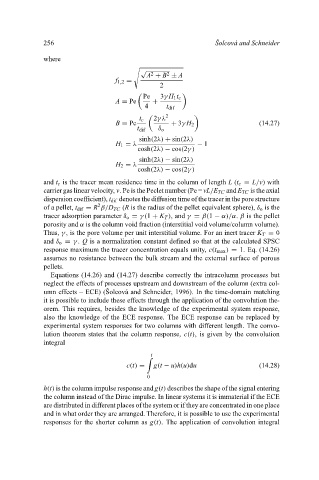
where
√
Šolcová and Schneider
2
2
A + B ± A
f 1,2 =
2

Pe 3γ H 1 t c
A = Pe +
4 t dif
2
t c 2γλ
B = Pe + 3γ H 2 (14.27)
t dif δ o
sinh(2λ) + sin(2λ)
H 1 = λ − 1
cosh(2λ) − cos(2γ)
sinh(2λ) − sin(2λ)
H 2 = λ
cosh(2λ) − cos(2γ)
and t c is the tracer mean residence time in the column of length L (t c = L/v) with
carrier gas linear velocity, v. Pe is the Peclet number (Pe = vL/E TC and E TC is the axial
dispersion coefficient), t dif denotes the diffusion time of the tracer in the pore structure
2
of a pellet, t dif = R β/D TC (R is the radius of the pellet equivalent sphere), δ o is the
tracer adsorption parameter δ o = γ(1 + K T ), and γ = β(1 − α)/α. β is the pellet
porosity and α is the column void fraction (interstitial void volume/column volume).
Thus, γ , is the pore volume per unit interstitial volume. For an inert tracer K T = 0
and δ o = γ . Q is a normalization constant defined so that at the calculated SPSC
response maximum the tracer concentration equals unity, c(t max ) = 1. Eq. (14.26)
assumes no resistance between the bulk stream and the external surface of porous
pellets.
Equations (14.26) and (14.27) describe correctly the intracolumn processes but
neglect the effects of processes upstream and downstream of the column (extra col-
umn effects – ECE) (Šolcová and Schneider, 1996). In the time-domain matching
it is possible to include these effects through the application of the convolution the-
orem. This requires, besides the knowledge of the experimental system response,
also the knowledge of the ECE response. The ECE response can be replaced by
experimental system responses for two columns with different length. The convo-
lution theorem states that the column response, c(t), is given by the convolution
integral
t

c(t) = g(t − u)h(u)du (14.28)
0
h(t) is the column impulse response and g(t) describes the shape of the signal entering
the column instead of the Dirac impulse. In linear systems it is immaterial if the ECE
are distributed in different places of the system or if they are concentrated in one place
and in what order they are arranged. Therefore, it is possible to use the experimental
responses for the shorter column as g(t). The application of convolution integral