Page 286 - gas transport in porous media

Chapter 16: Analyzing Barometric Pumping
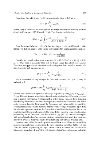
Combining Eqs. (16.8) and (16.9), the equation for flow is defined as:
k r 283
Q = 2πb S wb G(τ) (16.10)
µ g
where G(τ) is known as the flowing well discharge function for nonleaky aquifers
(Jacob and Lohman, 1952; Hantush, 1964). This function is defined as:

∞

4 −τu 2 1 du
G(τ) = e (16.11)
2
2
π 2 J (u) + Y (u) u
0
0
u=0
From Jacob and Lohman (1952), Carslaw and Jaeger (1959), and Hantush (1964),
it is known that for large τ, G(τ) can be approximated by a simpler representation:
2
For τ> 500, G(τ) ≈
ln(2.25τ)
2
Considering typical vadose zone properties (k r = 10 E-12 m , ϕ = 0.4, S g = 0.10,
r w = 0.0254 m), τ is greater than 500 for times larger than about 0.25 second.
Therefore, the approximate solution for calculating flow from a well as a result of a
step change in well gas pressure is:
k r 2
Q(t) = 2πb S wb (16.12)
µ g ln(2.25τ)
For a succession of step changes in flow and pressure, Eq. (16.12) may be
replaced with

k r 2
Q n (t) = 2πb S wb (k) (16.13)
t k
µ g ln 2.25τ 1 −
t
where n and k are flow and pressure time steps respectively and S wb (k) = P atm (t k )−
P z (t k ). This solution can be used directly with surface/subsurface differential pressure
data to predict flow from a well screened in a flow zone. The code for a computer
model using this solution has been developed and requires surface/subsurface differ-
ential pressure data, the thickness of the flow zone, well radius, radial permeability,
volumetric moisture content, porosity, and the yearly average pressure as input. Like
the subsurface pressure solution, the flow solution is calibrated using field data to cal-
culate the best fit for a single permeability value. In this case, the value is k r , the radial
permeability of the formation. The flow solution (Eq. (16.13)) can also be coupled
with an analytical subsurface pressure solution. Using these two analytical solutions,
flow from a vadose zone well can be predicted using only surface pressure data.
In many cases, all of the model parameters will not be available so a sensitivity
analysis was performed to determine the most important variables. Table 16.1 and
Table 16.2 show, respectively, the input values used in the model and the results of
this sensitivity analysis. From Table 16.2 it is clear that differential pressure and radial