Page 154 - Geochemical Anomaly and Mineral Prospectivity Mapping in GIS

Analysis of Geologic Controls on Mineral Occurrence 155

scales of the fractal systems interpreted from the results of the two methods are similar.
Discrepancies in fractal dimensions estimated via the box-counting method and the
radial-density method are difficult to explain, although, according to Carlson (1991),
such inconsistencies commonly occur in measuring fractal dimensions. For example, in
estimating the radial-density of points in a raster-based GIS, there is no rule-of-thumb
for choosing an ideal pixel size except that one should apply sound reasoning related to
the geo-objects represented by the points. The results of the box-counting and the radial-
density fractal analyses of the spatial distribution of the occurrences of epithermal Au
deposits in the Aroroy district commonly imply, however, that certain types of controls
are operating on at least two scales (lengths, widths, or diameters). One type of control
(e.g., fracture systems) possibly operates at scales of at most 2.8 km, which is plausibly
at the ‘deposit-to-another-deposit’ scale. The other type of control (e.g., hydrothermal
systems) possibly operates at scales of at least 7 km, which is plausibly at the scale of a
mineralised landscape (i.e., district scale in this case). These interpretations can be
investigated further via the application of Fry analysis

Fry analysis
Fry analysis (Fry, 1979), which is a geometrical method of spatial autocorrelation
analysis of a type of point geo-objects, is another useful technique to study spatial
distribution of points representing occurrences of mineral deposits of the type sought.
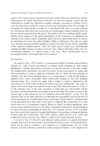
The method plots translations (so-called Fry plots) of point geo-objects by using each
and every point as a centre or origin for translation. Fig. 6-5 shows the basic principle in
creating a Fry plot using analogue maps (e.g., tracing paper). A map of data points is
marked with a series of parallel (either north-south trending or east-west trending)
reference lines. On a second but empty map, a centre or origin is indicated by the
intersection of a north-south trending line and an east-west trending line. The centre or
origin in the second map is then placed on top of one of the data points (point 1 in Fig. 6-
5), the reference lines of the same directions in both maps are kept parallel and the
positions of all the data points are recorded in the second map. The centre or origin in the
second map is then placed on top of a different data point (point 2 in Fig. 6-5), the
reference lines of the same directions in both maps are kept parallel and the positions of
all the data points are recorded again in the second map. The procedure is continued until
all the data points have been used as the centre or origin in the second map. For n data
2
points there are n -n translations created. These are called ‘all-object-separations’ plots
and are more commonly known as ‘Fry plots’, developed originally for the investigation
of strain and strain partitioning in rocks (Fry, 1979; Hanna and Fry, 1979). Fry plots
have been used in the analysis of spatial distributions of occurrences of mineral deposits
(Vearncombe and Vearncombe, 1999, 2002; Stubley, 2004; Kreuzer et al., 2007) and
geothermal fields (Carranza et al., 2008c) in order to infer their structural controls.
It is clear in Fig. 6-5 that a Fry plot enhances subtle patterns in a spatial distribution
of points and it also records distances and orientations between pairs of translated points,
which can be used to construct a rose diagram as a complementary tool for visual
analysis of trends reflecting controls by certain geological features. A rose diagram can