Page 199 - Geochemical Anomaly and Mineral Prospectivity Mapping in GIS

Knowledge-Driven Modeling of Mineral Prospectivity 201

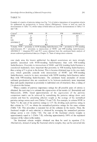
TABLE 7-I

Example of a matrix of pairwise ratings (see Fig. 7-6) of relative importance of recognition criteria
for epithermal Au prospectivity in Aroroy district (Philippines). Values in bold are used for
demonstration in Table 7-II, whilst values in bold italics are used for demonstrations in Tables 7-II
and 7-III.

Criteria 1 NNW FI NW ANOMALY
NNW 1 5 6 1/2
FI 1/5 1 5 1/2
NW 1/6 1/5 1 1/2
ANOMALY 2 2 2 1
Sum 2 3.37 8.2 14 2.5
1 Criteria: NNW = proximity to NNW-trending faults/fractures; NW = proximity to NW-trending
faults/fractures; FI = proximity to intersections of NNW- and NW-trending faults/fractures:
ANOMALY = integrated PC2 and PC3 scores obtained from the catchment basin analysis of
2
stream sediment geochemical data (see Chapter 3). Sum of ratings down columns.

case study area, the known epithermal Au deposit occurrences are more strongly
spatially associated with NNW-trending faults/fractures than with NW-trending
faults/fractures. Proximity to intersections of NNW- and NW-trending faults/fractures is
considered moderately more important that proximity to NW-trending faults/fractures;
thus a rating of 5 is given to the former. This is because dilational jogs in the case study
area, which generally coincide with intersections of NNW- and NW-trending
faults/fractures, seem to be more associated with NNW-trending faults/fractures rather
than with NW-trending faults/fractures. The catchment basin anomalies of stream
sediment geochemical data are considered to be between moderately more important
than and equally important as proximity to individual sets of structures; thus, a rating of
2 is given to the former.
When a matrix of pairwise importance ratings for all possible pairs of criteria is
obtained, the next step is to estimate the eigenvectors of the matrix (cf. Boroushaki and
Malczewski, 2008). Good approximations of the eigenvectors of the pairwise
comparison matrix can be achieved by normalising the pairwise ratings down each
column and then by calculating criterion weight as the average of the normalised
pairwise ratings across each row (Tables 7-I and 7-II). For example, in column NNW in
Table 7-I, the sum of the pairwise ratings is 3.37. By dividing each pairwise rating in
that column by 3.37, we obtain the normalised pairwise ratings for the same column
(Table 7-II). This procedure is repeated for all the columns in the matrix. Then, the
fractional weight of each criterion is obtained by averaging the normalised pairwise
ratings across a row (Table 7-II). The sum of the fractional criteria weights is
approximately equal to 1 (Table 7-II), reflecting approximately 100% of the explained
variance of the values in the matrix.
The fractional criteria weights obtained can then be used in equation (7.1).
Alternatively, instead of using the fractional criteria weights, they can be converted into