Page 43 - Geochemical Anomaly and Mineral Prospectivity Mapping in GIS

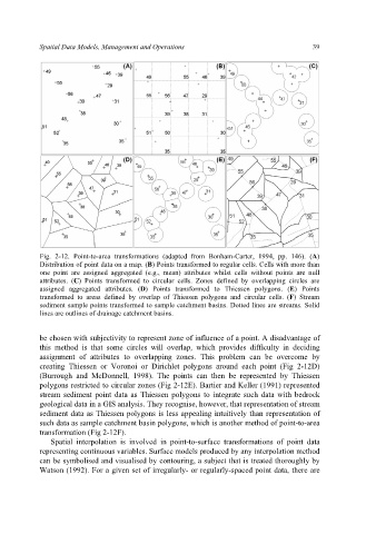
Spatial Data Models, Management and Operations 39

Fig. 2-12. Point-to-area transformations (adapted from Bonham-Carter, 1994, pp. 146). (A)
Distribution of point data on a map. (B) Points transformed to regular cells. Cells with more than
one point are assigned aggregated (e.g., mean) attributes whilst cells without points are null
attributes. (C) Points transformed to circular cells. Zones defined by overlapping circles are
assigned aggregated attributes. (D) Points transformed to Thiessen polygons. (E) Points
transformed to areas defined by overlap of Thiessen polygons and circular cells. (F) Stream
sediment sample points transformed to sample catchment basins. Dotted lines are streams. Solid
lines are outlines of drainage catchment basins.

be chosen with subjectivity to represent zone of influence of a point. A disadvantage of
this method is that some circles will overlap, which provides difficulty in deciding
assignment of attributes to overlapping zones. This problem can be overcome by
creating Thiessen or Voronoi or Dirichlet polygons around each point (Fig 2-12D)
(Burrough and McDonnell, 1998). The points can then be represented by Thiessen
polygons restricted to circular zones (Fig 2-12E). Bartier and Keller (1991) represented
stream sediment point data as Thiessen polygons to integrate such data with bedrock
geological data in a GIS analysis. They recognise, however, that representation of stream
sediment data as Thiessen polygons is less appealing intuitively than representation of
such data as sample catchment basin polygons, which is another method of point-to-area
transformation (Fig 2-12F).
Spatial interpolation is involved in point-to-surface transformations of point data
representing continuous variables. Surface models produced by any interpolation method
can be symbolised and visualised by contouring, a subject that is treated thoroughly by
Watson (1992). For a given set of irregularly- or regularly-spaced point data, there are