Page 44 - Geochemical Anomaly and Mineral Prospectivity Mapping in GIS

40 Chapter 2

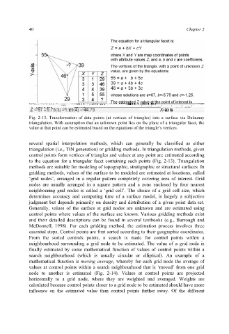
Fig. 2-13. Transformation of data points (at vertices of triangles) into a surface via Delaunay
triangulation. With assumption that an unknown point lies on the plane of a triangular facet, the
value at that point can be estimated based on the equations of the triangle’s vertices.

several spatial interpolation methods, which can generally be classified as either
triangulation (i.e., TIN generation) or gridding methods. In triangulation methods, given
control points form vertices of triangles and values at any point are estimated according
to the equation for a triangular facet containing such points (Fig. 2-13). Triangulation
methods are suitable for modeling of topographic, stratigraphic or structural surfaces. In
gridding methods, values of the surface to be modeled are estimated at locations, called
‘grid nodes’, arranged in a regular pattern completely covering area of interest. Grid
nodes are usually arranged in a square pattern and a zone enclosed by four nearest
neighbouring grid nodes is called a ‘grid cell’. The choice of a grid cell size, which
determines accuracy and computing time of a surface model, is largely a subjective
judgment but depends primarily on density and distribution of a given point data set.
Generally, values of the surface at grid nodes are unknown and are estimated using
control points where values of the surface are known. Various gridding methods exist
and their detailed descriptions can be found in several textbooks (e.g., Burrough and
McDonnell, 1998). For each gridding method, the estimation process involves three
essential steps. Control points are first sorted according to their geographic coordinates.
From the sorted controls points, a search is made for control points within a
neighbourhood surrounding a grid node to be estimated. The value of a grid node is
finally estimated by some mathematical function of values of control points within a
search neighbourhood (which is usually circular or elliptical). An example of a
mathematical function is moving average, whereby for each grid node the average of
values at control points within a search neighbourhood that is ‘moved’ from one grid
node to another is estimated (Fig. 2-14). Values at control points are projected
horizontally to a grid node, where they are weighted and averaged. Weights are
calculated because control points closer to a grid node to be estimated should have more
influence on the estimated value than control points farther away. Of the different