Page 45 - Geochemical Anomaly and Mineral Prospectivity Mapping in GIS

Spatial Data Models, Management and Operations 41

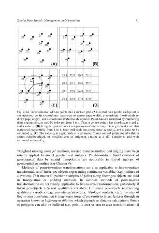
Fig. 2-14. Transformation of data points into a surface grid. (A) Control data points; each point is
characterised by its x-coordinate (east-west or across page width), y-coordinate (north-south or
down page length), and z-coordinate (value beside a point). Point data are identified by numbering
them sequentially, as read by software, from 1 to i. Thus, a control point i has coordinates x i and y i
and a value z i . (B) A regular grid of nodes is superimposed on the map. These grid nodes are also
numbered sequentially from 1 to k. Each grid node has coordinates x k and y k , and a value to be
estimated z k . (C) The value z k at a grid node k is estimated from n control points found within a
search neighbourhood, of specified area of influence, centred at k. (D) Completed grid with
estimated values of z k .

‘weighted moving average’ methods, inverse distance method and kriging have been
usually applied to model geochemical surfaces. Point-to-surface transformations of
geochemical data by spatial interpolation are applicable in fractal analysis of
geochemical anomalies (see Chapter 4).
Methods of point-to-surface transformations are also applicable to line-to-surface
transformations of linear geo-objects representing continuous variables (e.g., isolines of
elevation). That means all points or samples of points along linear geo-objects are used
in triangulation or gridding methods. In contrast, methods of point-to-area
transformations are not readily applicable to line-to-area transformations, particularly if
linear geo-objects represent qualitative variables. For linear geo-objects representing
qualitative variables (e.g., curvi-linear structures, lithologic contacts, etc.), the idea of
line-to-area transformation is to generate zones of proximity to linear features through an
operation known as buffering or dilation, which depends on distance calculations. Points
or polygons can also be buffered (i.e., point-to-area or area-to-area transformations) if