Page 125 - Industrial Power Engineering and Applications Handbook

6/106 Industrial Power Engineering and Applications Handbook

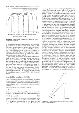
Nearly constant torque speed I load (torque). For instance, referring to Figure 6.9, the
control with ver! smaller the load I,,, the smaller will be sin 8, and the
larger the load Ia2, the larger will be sin &. Thus to
achieve a required level of speed control the stator current,
I,, field current, I,,,, and phasor angle, 8, can be suitably
varied. Since it is the phasor of the rotor flux (rotating
field), i.e. the magnitude and its angular position with
respect to the active current of the stator, which is being
varied, to achieve the required speed control, this phasor
control is called field oriented control (FOC). The theory
of field orientation was first introduced by F. Blaschke
in 1972 (see Blascke (1972) and EPE Journal (1991)).
Having been able to identify the rotor field phasor it is
now possible to vary this and obtain a speed control in a
squirrel cage machine similar to that in a d.c. machine.
For field-oriented controls, a mathematical model of
Frequency (Speed) -
012 5 10 20 30 40 50 60Hz the machine is developed in terms of rotating field to
Below the base speed t+----) Above the base speed represent its operating parameters such as N,, I,, I, and
8 and all parameters that can influence the performance
of the machine. The actual operating quantities are then
Figure 6.8 Speed-torque characteristics by flux (I,,,) control computed in terms of rotating field and corrected to the
(single phasor control)
required level through open- or closed-loop control
schemes to achieve very precise speed control. To make
to vary the speed of the machine by sensing the component, the model similar to that for a d.c. machine, equation
I,, of the machine. Any variation in the actual I,,, than (6.2) is further resolved into two components, one direct
the desired pre-set value in the inverter switching logistics axis and the other quadrature axis, as discussed later.
is made up by the PWM technique. The field-oriented Now it is possible to monitor and vary these components
block diagram illustrated in Figure 6.12 below can be individually, as with a d.c. machine. With this phasor
suitably simplified for I, control. Tachogenerator or pulse control we can now achieve a high dynamic performance
encoder feedback devices can be employed to achieve and accuracy of speed control in an a.c. machine, similar
higher accuracy in speed control. to a separately excited d.c. machine. A d.c. machine
With years of research and development in the field of provides extremely accurate speed control due to the
static drives, it is now possible to identify and separate independent controls of its field and armature currents.
these two parameters (I, and I,,,) and vary them Different manufacturers have adopted different methods
individually, as in a d.c. machine, to achieve extremely with minor changes to achieve almost the same objective.
accurate speed control, even slightly better than in d.c. For example, field-oriented control was first introduced
machines. In d.c. machines the armature current and the by Allen Bradley in the USA in 1981 and a similar
field strength are also varied independently. A.C. machines technique was introduced at the same time by ABB of
can now be used to provide very precise speed control, Finland. ABB claim their technique to he still faster in
as accurate as +_ 0.001% of the set speed, with closed- responding, as it eliminates the modulation section of
loop feedback controls. This technique of speed control
is termed field-oriented control (FOC) and is discussed
below.

6.4.2 Field-oriented control (FOC)
This is commonly known as double phasor or phasor
(vector) control. If we analyse equation (1.1) in Chapter
1 we will observe that @is a function of stator magnetizing
current, I,, and I, is a transformation of the stator active
current, I,.
Hence, equation (1.1) can be rewritten as
T oc I, '7,

Both of them are phasor quantities, and are shown in
Figure 6.9. In absolute terms, they can be represented by
T = k . I, . I, sin 8 (6.2)
where 8 represents the electrical position of the rotor
field in space with respect to the stator. In other words,
it is the- phasor displacement or slip angle between Figure 6.9 Phasor representation of field current (I,,,) and
I,,, andI, and will continue to vary with variation in stator active current (I,)