Page 183 - Integrated Wireless Propagation Models

I
M a c r o c e I P r e d i c t i o n M o d e I s - P a r t 2 : P o i n t - t o - P o i n t M o d e I s 161

- - - - - -

point
- -- -
.
.
___ ,_.. ... .... ��flective
plane
FIGURE 3.2.3.1 LOS.

:
�
35.oo �----�----�----�----�----�----�----�----�-----.
• • ••
• ••
,

.. ::.·
30.00 1----- -- +- -- -- -+- -- -- -+ -- -- ---1-- -- --.:�""�'..-= • •• • • • • ,;
25.00 1----- -- +- -- -- -+- -- -- -+ -- -- ---1-- -- . o"".:,'--+-- -- ----;c+---:- -- -+-- -- --+ -- -- ----1
·
i
w - � �
"'0 :
. .
,,
-� 20.00 r--- -- +- -- -- -+- -- -- -+ -- -- ----t----:-.�·,.._ -- +-- ----,.� .-t- , -- -- -+ -- -- --+ -- -- ----1
•
..r::.
C» 1 5 .00 1---- -- +- -- -- -+- -- � ... ,\ -- -+ -- -- ---l'-'---- -- --'-+--......:.... -- ii, ------; �1-!: -+-- -- --+-- -- ----1
� 0 _ ��
Cii 1 0 .00 1----- -- +- -- -- -+- -- �-+ -- -- ---1-- -- -- +----'- ' ,_;,;• +---.>'----+--- -- -+-- -- ---1
(ij . . 0 ,.. ":'-.-:,:
.'
� 5 00 . , , · . \0 •''-'-' ; .!'_ - -- -- +--- -- +- -- -- --1
' --+--
"�_....
•
U5 : · ·, · ·
,, . ... ... ,;:.� · .... . i . ,·� : : r.:::� :
;::;: . . .. . . . . ·�, .. :�·ii., "
o.oo , ... ,.; /.: z .. ;i; ::j � ·'4l! , , , . • . : . - : ··:H !'t �"ii-;";i)-.-: -;. �#l'"-.-,,1> -- +-- -c,,.;- .----+- -- -- -+ -- -- --+ -- -- ----1
;>-
,
.
· · · -� r �·-�·•"r· · · "'- • ' · · . · · . .
... · · . . · .
..
-5.00 :,; :· � I !\'¥: · •.
-1 0.00 L_ __ __ L_ __ __ � -- -- � -- -- � -- -- _L __ __ _L __ __ _L __ __ �-- -- �
1 . 00 1 0 .00
Distance (miles)
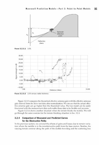
FIGURE 3.2.3.2 LOS versus radial distance.
Figure 3.2.3.3 compares the theoretical effective antenna gain with the effective antenna
gain derived from the drive test data after normalization. We can see that the actual effec­
tive antenna gain can go higher than the theoretical value. The Lee model can be easily
fine-tuned with the measurement data and enable those data to be flexible and accurate.
Figure 3.2.3.4 shows another situation when the terrain blocks the mobile. We will
go through the same exercise for the terrain blocking situation in Sec. 3.2.4
3.2.4 Comparison of Measured and Predicted Curves
for the Obstructive Paths
In the previous section, we covered the effects of gains and losses due to terrain varia­
tion where the mobile is in the nonobstructive path from the base station. Besides, the
varying terrain contour along the path of the mobile traveling and the scattering loss