Page 184 - Integrated Wireless Propagation Models

162 C h a p t e r T h r e e

20 ' · ............ .. ..... .

.
. �
. ..
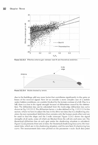
- - - Best fit
- - Theoretical line

-30 L-------L-------�------�------�------�
0 0.2 0.4 0.6 0.8

FIGURE 3.2.3.3 Effective antenna gai n between best-fit and theoretical prediction.

Knife
/ edge

Antenna k.

FIGURE 3.2.3.4 Mobile blocked by terra i n .

due to the buildings add one more factor that contributes significantly to the gains or
losses of the received signal. Now let us consider a more complex case of a mobile
under hidden conditions, or a mobile blocked by the terrain contour of a hill. Due to a
hill, there is a loss in the signal strength because of diffractions caused by the obstruc­
tion. The diffraction loss can be calculated from the knife-edge diffraction loss curve
shown in Fig. . 9.2.2.1.2. The diffraction factor, v, is also defined in Fig. . 9.2.2. . 2. In this
1
1
1
section, where we have to adjust the loss in the drive test data due to a shadowing situ­
ation, the new normalized field data then contains only the human-made effect and can
be used to find the slope and the 1-mile intercept. Figure 3.2.4.1 shows the signal
strengths of all spots, some of which are blocked from the cell site and some not. The
theoretical diffraction loss at each spot under the shadowing situation is calculated.
Figure 3.2.4.2 presents three sets of data: the theoretical shadowing loss curve; the mea­
sured data, which are in the shadowing situation; and the new best-fit shadowing loss
curve. The measurement data were plotted on the parameter v scale. Each data point