Page 185 - Integrated Wireless Propagation Models

I
M a c r o c e I P r e d i c t i o n M o d e I s - P a r t 2 : P o i n t - t o - P o i n t M o d e I s 163

20.00
1 5 .00
1 0 .00
co 5.00
"0 . . .. : .. : , · .
.. .
,.
.� 0.00 . . .
, : . . :rl,- . . � . , � · · . "'' ' • '
r-
_
:
_:..,
.
·
.
� -5.00 1---+,....--+--.......t- - -f-·..,.;_-=";.''-=:;"' ... -:-- . � � �+----l- - -f
-
� -1 0.00 1- - --+. ..::: · �· �-o: -+-- � ''lf 'r. ' -i- -.'f ::-- � -:+ - _,.: +- -· -" .·:_ +- - --+ - -1

- .. . ,, : :· ,.J:Yf.•" .!:I
t-:1
�
•
tl -1 5.00 i--:=! .,-:. -f"'Ti "r.- -+- ---: - . :·� f ! :· ··.:· ··· : . . . i - +- - --+ - - -l
-=;;j ;..._ � � ....... .__ +--
� -20.00 1-"·-:' . . �--+-:-'':·.,.-:..:.:.·:·-::�·';.:."'-:- ·;� ... :.:.'+�-.'�::-=""·.�,..· ·.'-i' _ _.·.r:-...:�·'":" - - +-- - +----+- - -1
. · · : ·
� -25.00 !- -· = ::. ., .:..:. :�-+ ·..:.. � - --!r !-· ·_ .· _ _ . . +- _- _ --1 - - +. +- - --+ - - -+ - - +- - --1
-30.00 1- --+-- � 1---+-- - f--. .,\',f---+- - 1---+---1

-35.00 1---+-----11---+---1--""t---t---+--t---1
-40.00 .__ _ _._ _ ___..__ _ _._ _ _ .___....�... _ _ .___....�... _ _ ...__....1
1 . 00 1 0 .00
Distance (miles)
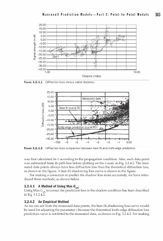
FIGURE 3.2.4.1 Diffraction loss versus radial distance.
20.00 ........ - - - - - -r - - - - - -r - - - - - ......
1 5 .00 -3-------+------+------4
1 0 .00 +- - - - - -+ -- � - =� - __. ........ ���
ill
� 5.00 -7-:-::--:---�f---.::"""':-:--.r_,
U)
.fl 0.00
§ -5.00 -T---��-+---.:...ao��p.a""=��
·� -10.00 -r - -; ;-:i ;; � � J; IJtlllfl(f
� -15.00 � - - - ..;.:!.-:�i-! � ..:;......;. .... .;;..� !-: �-:iiifi'� �
-20.00 -2""-.o;;.���;;.;;;;;�..;..,o;.;;.;..;...;;..;.,L._ � � ..... r::::o..---�
-25.00 t - - -:� :; � p. .... -��::..t- - - - -----1
-30.00 -:r--........;;.f-.,....""'Pf-.+,...........,t-1---...-+--�
-700 -6 -5 -4 -3 -2 -1 0.00
FIGURE 3.2.4.2 Diffraction loss comparison between best-fit and knife-edge prediction.
was first calculated its v according to the propagation condition. Also, each data point
was subtracted from its path loss before plotting on the v scale in Fig. 3.2.4.2. The mea­
sured data points always have less diffraction loss than the theoretical diffraction loss,
as shown in the figure. A best-fit shadowing loss curve is shown in the figure.
For making a correction to predict the shadow loss more accurately, we have intro­
duced three methods, as shown below.
3.2.4. 1 A Method of Using Max Getth
Using Max Geftll to correct the prediction loss in the shadow condition has been described
in Eq. 3.1.2.4.2.

3.2.4.2 An Empirical Method
As we can see from the measured data points, the best-fit shadowing loss curve would
be used for adjusting the parameter v because the theoretical knife-edge diffraction loss
prediction curve is not fitted to the measured data, as shown in Fig. 3.2.4.2. For making