Page 181 - Integrated Wireless Propagation Models

I
M a c r o c e I P r e d i c t i o n M o d e I s - P a r t 2 : P o i n t - t o - P o i n t M o d e I s 159

Normalization is done only on the valid measured points. After all measured points
have been normalized based on terrain, use the mean square best-fit algorithm to calcu­
late the slope and intercept for the cell site.
After inserting the proper path loss slope and the 1-mile intercept in Eq. (3.2.1.1),
the signal strength predictions can be found by adjusting Geffh or L(v) from a terrain
contour map.

3.2.2 Measurement Data Characteristics
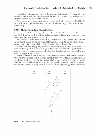
The measured data from a single cell were collected in the Italy Ivrea area. There are a
total of 10 drive routes. This cell site had an elevation of 246 m above sea level with a
50-m transmitter height and an ERP of 45.3 W.
The measured data were collected by driving away and toward the cell site.
Figure 3.2.2.1 shows the actual physical locations of these 10 routes, which demon­
strated most of the characteristics of the measured data at this cell site.
Because the morphology might be drastically different in making the same setup of
cell sites, it is important to be able to apply different slopes and intercepts for different
areas covered by the same setup of cell sites. This situation can easily be handled and
solved by applying this treatment.
When a cell site is located in a hilly area, there are some known terrain problems.
Also, morphology data, such as tunnels, elevated highways and bridge information, are
not always available. Usually, the measured data were collected without screening
these restrictions. Although there are questions regarding how accurate the measured
data are, the amount of sampled data is believed to be large enough to be statistically

45 · . 50 55
00 E · . . 00 E 00 E
. .
. .
. . .
· . · :
.
�:
.· · · . ; _ : . : - .
: .· . . .

0
. .
.: · ... · .
. . .. : . .
: , ; �: ·
: :_ ....... · ::

FIGURE 3.2.2.1 Measurement routes.