Page 186 - Integrated Wireless Propagation Models

164 C h a p t e r T h r e e

�
....
�1
�
-� 2
Pl
_]
.,
·.c
... ,

'
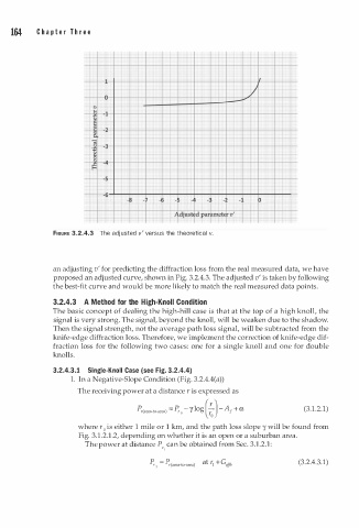
FIGURE 3.2.4.3 The adjusted v versus the theoretical v.

an adjusting v for predicting the diffraction loss from the real measured data, we have
'
proposed an adjusted curve, shown in Fig. 3.2.4.3. The adjusted v is taken by following
'
the best-fit curve and would be more likely to match the real measured data points.
3.2.4.3 A Method for the H i gh-Knoll Condition
The basic concept of dealing the high-hill case is that at the top of a high knoll, the
signal is very strong. The signal, beyond the knoll, will be weaken due to the shadow.
Then the signal strength, not the average path loss signal, will be subtracted from the
knife-edge diffraction loss. Therefore, we implement the correction of knife-edge dif­
fraction loss for the following two cases: one for a single knoll and one for double
knolls.
3.2.4. . 1 Single-Knoll Case (see Fig. 3.2.4.4)
3
1. In a Negative-Slope Condition (Fig. 3.2.4.4(a))
The receiving power at a distance r is expressed as
1
P, <area-to-areal = P,, - Y log (� J -A 1 + a (3. . 2.1)
where r0 is either 1 mile or 1 km, and the path loss slope y will be found from
Fig. 3.1.2.1.2, depending on whether it is an open or a suburban area.
The power at distance P can be obtained from Sec. 3.1.2.1:
'r
(3.2.4.3.1)