Page 333 - Integrated Wireless Propagation Models

I n - B u i l d i n g ( P i c o c e l l ) P r e d i c t i o n M o d e l s 311

l
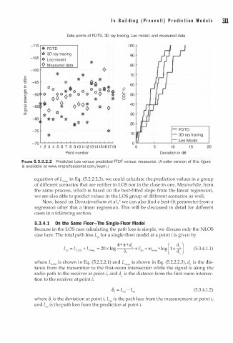
Data points of FDTD, 3D ray tracing, Lee mode , and measured data
-11 0 1 0 0
* FDTD
1l 3D ray tracing 90
-105 0 Lee model
0 Measured data * 80
-100 0
* * 70
E
((] * *
""0 -95 0 i �
-� 60
0
.r: O o • • 0 0 ° o 0 · � � -;?.
0, LL
c -90 0 0 0 0 * 0 0 0 0 50
� ¢ 0 * * 0
t5
(ij -as< 1>. � 0 o o � * 40
c �
Ol 0
i:i5 * * * 30
-80 * * * -t:
*
• * 20
-75 - FDTD
* 1 0 - 3D ray tracing
- Lee Model
-70 0
1 2 3 4 5 6 7 8 9 1 0 1 1 1 2 1 3 1 4 1 5 1 6 1 7 1 8 0 5 1 0 1 5 20
Point number Deviation in dB
FIGURE 5.3.3.2.2 Predicted Lee versus predicted FTDT versus measured. (A color version of this figure
is available at www.mhprofession l . c omjiwpm. )
a
equation of L, in Eq. (5.2.2.2.3), we could calculate the prediction values in a group
oom
of different scenarios that are neither in LOS nor in the close-in one. Meanwhile, from
the same process, which is based on the best-fitted slope from the linear regression,
we are also able to predict values in the LOS group of different scenarios as well.
Now, based on Devasirvatham et al.,8 we can also find a best-fit parameter from a
regression other that a linear regression. This will be discussed in detail for different
cases in a following section.

5.3.4. 1 On the Same Floor-The Single-Floor Model
Because in the LOS case calculating the path loss is simple, we discuss only the NLOS
case here. The total path loss L ; for a single-floor model at a point i is given by
p
d
4 * n * d ( )
* l
+
L i = L ws , + L room, = 20 X log A '• + �OS mroom og 1 + :: (5.3.4.1.1)
p
d
where L ws is shown in Eq. (5.2.2.2.1) and L, is shown in Eq. (5.2.2.2.3), d ; is the dis­
oom
,
tance from the transmitter to the first-room intersection while the signal is along the
radio path to the receiver at point i, and d ; is the distance from the first room intersec-
'
tion to the receiver at point i:
(5.3.4.1.2)
where o; is the deviation at point i, L is the path loss from the measurement at point i,
mi
and L ; is the path loss from the prediction at point i.
p