Page 334 - Integrated Wireless Propagation Models

312 C h a p t e r F i v e

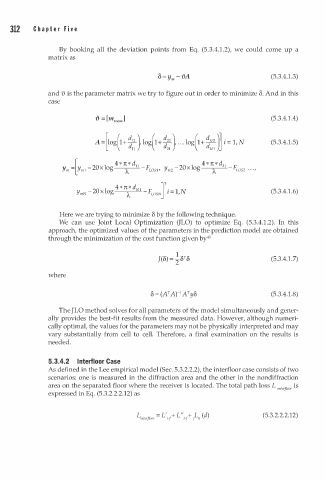
By booking all the deviation points from Eq. (5.3.4.1.2), we could come up a
matrix as

(5.3.4.1.3)

and � is the parameter matrix we try to figure out in order to minimize 8. And in this
case

.
= [ ] (5.3.4 1 . 4)
i}- mroom
A =[ log(1 + ), log(1 + dzz l . . . log(1 + )� i = 1, N (5.3.4.1.5)
d
d12
Nz
dll d21 J d 1
N �
4 * 7t * d 11 4 * 1t * d 21
Ym = Ym 1 - 2 0 xlog A F OSl' y m2 -20 X log A Fws z · · . ,
[
L
] T
N
1
- 1,N
YmN - 2 Q xlog 4 * 1t * d 1 - FwsN l - (5.3.4. . 6)
·
A
Here we are trying to minimize o by the following technique.
1
We can use Joint Local Optimization (JLO) to optimize Eq. (5.3.4. . 2). In this
approach, the optimized values of the parameters in the prediction model are obtained
through the minimization of the cost function given by4 0
(5.3.4.1.7)

where

1
o = ( N A)- Ny8 (5.3.4.1.8)
The JLO method solves for all parameters of the model simultaneously and gener­
ally provides the best-fit results from the measured data. However, although numeri­
cally optimal, the values for the parameters may not be physically interpreted and may
vary substantially from cell to cell. Therefore, a final examination on the results is
needed.

5.3.4.2 lnterfloor Case
As defined in the Lee empirical model (Sec. 5.3.2.2.2), the interfloor case consists of two
scenarios: one is measured in the diffraction area and the other in the nondiffraction
area on the separated floor where the receiver is located. The total path loss L interfloor is
expressed in Eq. (5.3.2.2.2.12) as

'
L. fl = L . + L". + L (d) (5.3.2.2.2.12)
mter oor 1- 1 1- 1 1 11