Page 46 - Integrated Wireless Propagation Models

24 C h a p t e r O n e

99.9 0.1
99.0 1.0
96.0 4.0
94.0 6.0
90.0 10.0
80.0 20.0
70.0 30.0
60.0 40.0
50.0 50.0
40.0 60.0
30.0 70.0
ctl ctl
Vl 20.0 80.0 Vl
Vl Vl
·c; ·c;
Vl Vl
.0 .0
ctl 10.0 90.0 ctl
v v
Q) Q)
""0 ""0
. .e 5.0 95.0 . .e
0. 0.
E E
ctl ctl
Cii Cii
£ 2.0 96.0 £
g g
ii ii
ctl 1.0 99.0 ctl
.0 .0
e e
Cl. Cl.
"E 0.5 99.5 "E
Q) Q)
� �
Q) Q)
CL CL
0.2 99.8
0.1 99.9
0.05 99.95
99.98
99.99
l
Signal level, dB with spect to RMS ue, ,f2(
re
a
v
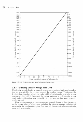
FIGURE 1.8.1.1 Statistical properties of a Rayleigh-fading signa . l
1.8.3 Estimating Unbiased Average Noise Level
Usually, the sampled noise in a mobile environment contains high-level impulses
2 2
that are generated by the ignition noise of the gasoline engine. 8• 9 Although the
p
level of these impulses is high, the u lse width of each impulse generally is very
narrow (see Fig. . 8.3. ) . As a result, the energy contained in each impulse is very
1
1
small and should not have any noticeable effect on changing the average power in
a 0.5-s interval.
However, in a normal situation, averaging a sampled noise is done by adding
up the power values of all samples, including the impulse samples, and dividing
the sum by the number of samples. This is called the conventionally averaged noise
power and is denoted nc.