Page 48 - Integrated Wireless Propagation Models

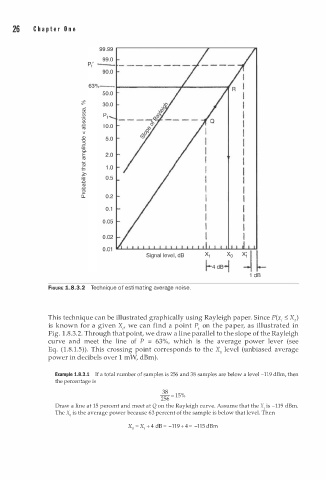
26 C h a p t e r 0 n e

�
0
cri
(/)
(/)
"(5 p t
(/)
.0
crl
v
Q)
""0
.�
c..
E
crl
iii
£
g
:0
crl
.0
e
(L

Signal level, dB

1 dB
FtGURE 1.8.3.2 Technique of estimating average noise.

This technique can be illustrated graphically using Rayleigh paper. Since P(x ; :<;; X,)
p
is known for a given X ,, we can find a o int P, on the pap r , s illustrated in
a
e
1
p
Fig. . 8.3.2. Through that point, we draw a line a rallel to the slope of the Rayleigh
curve and meet the line of P = 63%, which is the average p o wer lever (see
Eq. ( 1 . 8 . 1 . 5)). This crossing point corresponds to the X 0 level (unbiased average
p o wer in decibels over 1 m W, dBm).
Example 1.8.3.1 If a total number of samples is 256 and 3 8 samples are below a level -119 dBm, then
the percentage is
8
; = 1 5%
56
Draw a line at 15 percent and meet at Q on the Rayleigh curve. Assume that the X, is -119 dBm.
The X0 is the average power because 63 percent of the sample is below that level. Then
X0 = X , + 4 dB = -119 + 4 = -115 dBm