Page 49 - Integrated Wireless Propagation Models

I n t r o d u c t i o n t o M o d e l i n g M o b i l e S i g n a l s i n W i r e l e s s C o m m u n i c a t i o n s 27

Example 1.8.3.2 The total number of samples is 256. Three noise spikes are 20 dB above the normal
average. Find the errors, using the following two methods. Compare the results.
Use geometric average method. Let the power value of each sample (of 253 samples) after normalization
be 1; that is, the average is 1. Then the measured average of 256 samples, including three spikes, is
"" 253 ""
L.., X; + 100 L.., ' X;
N0 = M easured average = 1 1 2.16 (assume x; = 1)
256
= 3.3 dB above the true average
Statistical average method

63% of samples = 256 x 0.63 = 161 samples
This means that 161 samples should be under the average power level. Now three noise spikes added
to the 161 samples increases the number of samples to 164:

;� = 6 4%
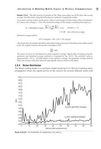
The power levels at 63 and 64 percent show almost no change. Typical data averaging using the
geometric and statistical average methods is illustrated in Fig. 1 . 8 .3.3. The corrected value is
approximately -11 8 to -119 dBm based on the statistical average. The geometric average method
biases the average value and causes an unacceptable error, as shown in the figure.
1.8.4 Rician Distribution
The Rician fading model is a stochastic model made by S. 0. Rice for studying radio
propagation when the signal arrives at the receiver by several different paths and

1 0 5
1 0 6
1 0 7
1 0 8
1 0 9
1 1 0
1 1 1
1 1 2
E
Ill
"0 1 1 3
1 1 4
1 1 5
1 1 6
1 1 7
1 1 8
1 1 9

Record (256 sample/record)
i
FIGURE 1.8.3.3 An l l u stration of comparison of N0 with X0.