Page 237 - System on Package_ Miniaturization of the Entire System

Mixed-Signal (SOP) Design 211

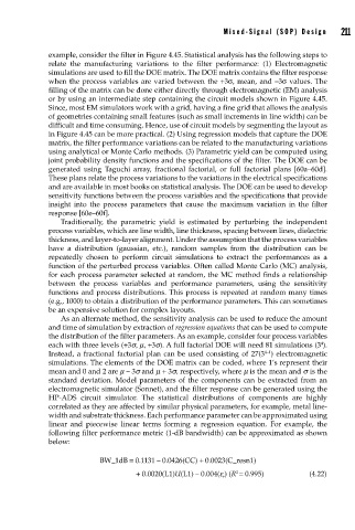
example, consider the filter in Figure 4.45. Statistical analysis has the following steps to
relate the manufacturing variations to the filter performance: (1) Electromagnetic
simulations are used to fill the DOE matrix. The DOE matrix contains the filter response
when the process variables are varied between the +3σ, mean, and –3σ values. The
filling of the matrix can be done either directly through electromagnetic (EM) analysis
or by using an intermediate step containing the circuit models shown in Figure 4.45.
Since, most EM simulators work with a grid, having a fine grid that allows the analysis
of geometries containing small features (such as small increments in line width) can be
difficult and time consuming. Hence, use of circuit models by segmenting the layout as
in Figure 4.45 can be more practical. (2) Using regression models that capture the DOE
matrix, the filter performance variations can be related to the manufacturing variations
using analytical or Monte Carlo methods. (3) Parametric yield can be computed using
joint probability density functions and the specifications of the filter. The DOE can be
generated using Taguchi array, fractional factorial, or full factorial plans [60a–60d].
These plans relate the process variations to the variations in the electrical specifications
and are available in most books on statistical analysis. The DOE can be used to develop
sensitivity functions between the process variables and the specifications that provide
insight into the process parameters that cause the maximum variation in the filter
response [60e–60f].
Traditionally, the parametric yield is estimated by perturbing the independent
process variables, which are line width, line thickness, spacing between lines, dielectric
thickness, and layer-to-layer alignment. Under the assumption that the process variables
have a distribution (gaussian, etc.), random samples from the distribution can be
repeatedly chosen to perform circuit simulations to extract the performances as a
function of the perturbed process variables. Often called Monte Carlo (MC) analysis,
for each process parameter selected at random, the MC method finds a relationship
between the process variables and performance parameters, using the sensitivity
functions and process distributions. This process is repeated at random many times
(e.g., 1000) to obtain a distribution of the performance parameters. This can sometimes
be an expensive solution for complex layouts.
As an alternate method, the sensitivity analysis can be used to reduce the amount
and time of simulation by extraction of regression equations that can be used to compute
the distribution of the filter parameters. As an example, consider four process variables
4
each with three levels (+3s, m, +3s). A full factorial DOE will need 81 simulations (3 ).
4–1
Instead, a fractional factorial plan can be used consisting of 27(3 ) electromagnetic
simulations. The elements of the DOE matrix can be coded, where 1’s represent their
mean and 0 and 2 are m – 3s and m + 3s, respectively, where m is the mean and s is the
standard deviation. Model parameters of the components can be extracted from an
electromagnetic simulator (Sonnet), and the filter response can be generated using the
HP-ADS circuit simulator. The statistical distributions of components are highly
correlated as they are affected by similar physical parameters, for example, metal line-
width and substrate thickness. Each performance parameter can be approximated using
linear and piecewise linear terms forming a regression equation. For example, the
following filter performance metric (1-dB bandwidth) can be approximated as shown
below:

BW_1dB = 0.1131 – 0.0426(CC) + 0.0023(C_resn1)
+ 0.0020(L1)U(L1) – 0.004(e ) (R = 0.995) (4.22)
2
r